Practical ML: Detecting Out-of-Distribution Data

Recently I worked on a project triangulating geo-coordinates of signals based on registrations in a radio network. Attempting to improve on traditional optimization based trilateration, I turned to neural networks to pick up subtle patterns in the underlying data space (ex: terrain in certain regions affects observed signal strength). This approach outperformed existing trilateration algorithms but suffered from high variance in the prediction quality. Most of the problematic predictions stemmed from samples that were not represented well in the original training data. This example highlighted a common problem in applied ML.

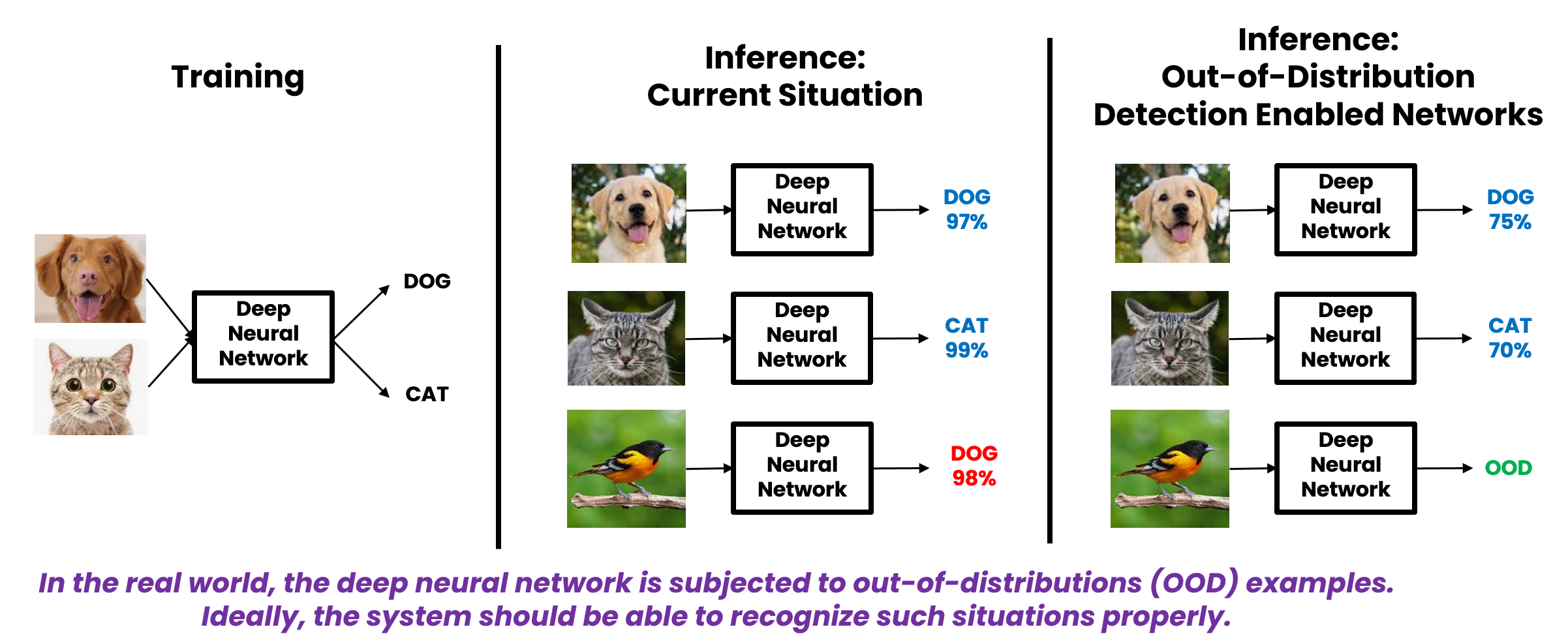
Wouldn’t it be nice if we could improve confidence in our predictions by detecting cases where new data differs significantly from the training distribution. One way to formalize this is Out-of-Distribution detection. See borrowed image below.

For the triangulation problem described above, I turned to a slick solution introduced in the paper: Distinction Maximization Loss, which describes a drop-in replacement to a typical softmax layer and a Max-Mean Logit Entropy Score that can be used to better detect “Out-of-Distribution” samples at inference time.

Implementing DisMax

The authors provide some code, but I was not able to get their implementations working. Instead I implemented the basics and created the following example to demonstrate the approach.

DisMax is comprised of a replacement for the classification layer in a model and a replacement for the cross entropy loss used to train the model. A minimal implementation below:

class DisMaxLossFirstPart(nn.Module):
    """This part replaces the model classifier output layer nn.Linear()."""

    def __init__(self, num_features: int, num_classes: int, temperature: float = 1.0):
        super(DisMaxLossFirstPart, self).__init__()
        self.num_features = num_features
        self.num_classes = num_classes
        self.distance_scale = nn.Parameter(torch.Tensor(1))
        nn.init.constant_(self.distance_scale, 1.0)
        self.prototypes = nn.Parameter(torch.Tensor(num_classes, num_features))
        nn.init.normal_(self.prototypes, mean=0.0, std=1.0)
        self.temperature = nn.Parameter(
            torch.tensor([temperature]), requires_grad=False
        )
    
    def forward(self, features: Tensor) -> Tensor:
        distances_from_normalized_vectors = torch.cdist(
            F.normalize(features),
            F.normalize(self.prototypes),
            p=2.0,
            compute_mode="donot_use_mm_for_euclid_dist",
        ) / math.sqrt(2.0)
        isometric_distances = (
            torch.abs(self.distance_scale) * distances_from_normalized_vectors
        )
        logits = -(isometric_distances + isometric_distances.mean(dim=1, keepdim=True))
        return logits / self.temperature

    def extra_repr(self) -> str:
        return "num_features={}, num_classes={}".format(
            self.num_features, self.num_classes
        )

class DisMaxLossSecondPart(nn.Module):
    """This part replaces the nn.CrossEntropyLoss()"""

    def __init__(self, model_classifier):
        super(DisMaxLossSecondPart, self).__init__()
        self.model_classifier = model_classifier
        self.entropic_scale = 10.0
        self.alpha = 1.0

    def forward(self, logits: Tensor, targets: Tensor) -> Tensor:
        batch_size = logits.size(0)
        probabilities = (
            nn.Softmax(dim=1)(self.entropic_scale * logits)
            if self.model_classifier.training
            else nn.Softmax(dim=1)(logits)
        )
        probabilities_at_targets = probabilities[range(batch_size), targets]
        loss = -torch.log(probabilities_at_targets).mean()
        return loss

Training a model w/ the DisMax layer and loss is simple - nothing fancy here:

model = ...
criterion = DisMaxLossSecondPart(model.classifier)
...

for i in range(TRAIN_STEPS):
  ...
  # Predict coordinates and evaluate loss
  outputs = model(Xtr)
  loss = criterion(outputs, Ytr)
  # Backward pass
  optimizer.zero_grad()
  loss.backward()
  optimizer.step()

Implementing Maximum Mean Logit Entropy Score

Implementing the MMLE score is very simple. I chose to use numpy here for simplicity in the plots to come.

from scipy.special import softmax as softmax_np
def mmles_np(logits: npt.NDArray) -> npt.NDArray:
    """Maximum Mean Logit Entropy Score"""
    probabilities = softmax_np(logits, axis=1)
    return (
        logits.max(1) + logits.mean(1) + (probabilities * np.log(probabilities)).sum(1)
    )

Here logits can be used to calculate not only softmax scores (traditional) but also MMLE scores which we’ll compare in the next section.

Does it work?

To demonstrate the use, I first generate some simple 2D data to represent ~200 “In-Distribution” classes and 1 very “Out-of-Distribution” class.

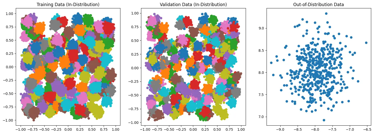Note the difference in the axes of the OOD data

Then I train and calibrate the model (see full notebook for details), before predicting on two different sets of data:

• held out validation dataset (In-Distribution)
• held out validation dataset (Out-of-Distribution)

For both sets I calculate the softmax scores (traditional) and the MMLE scores.

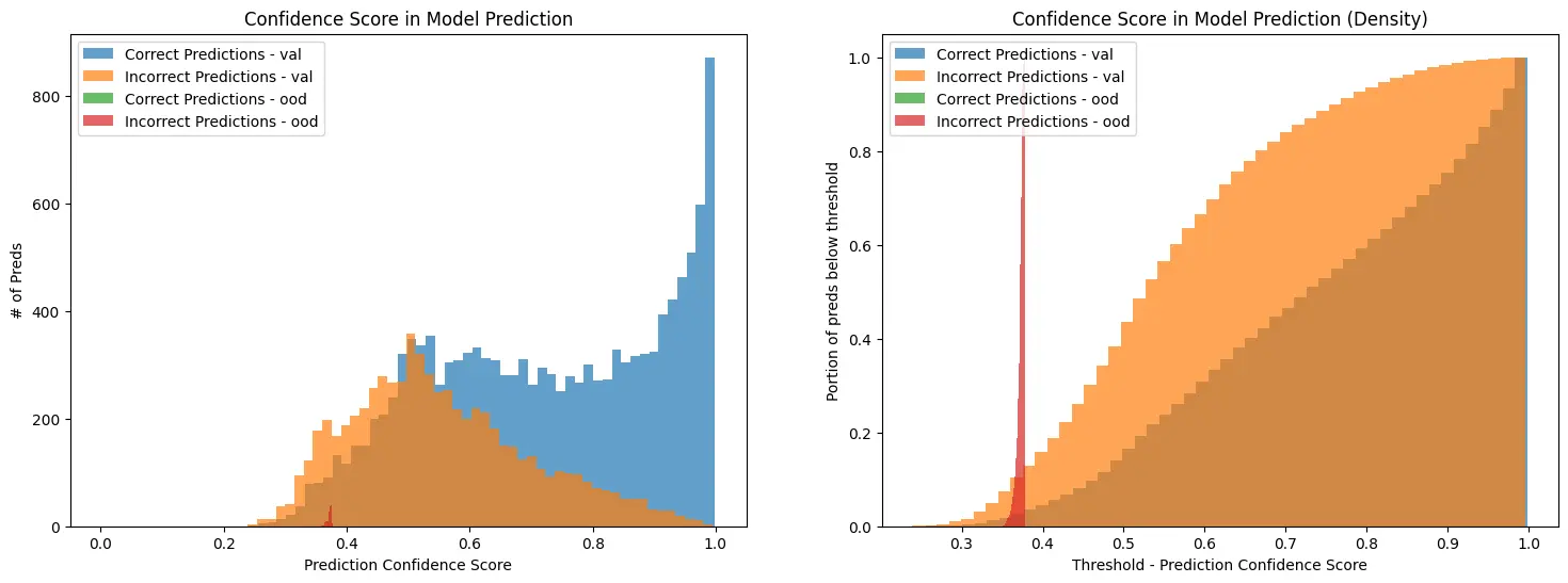
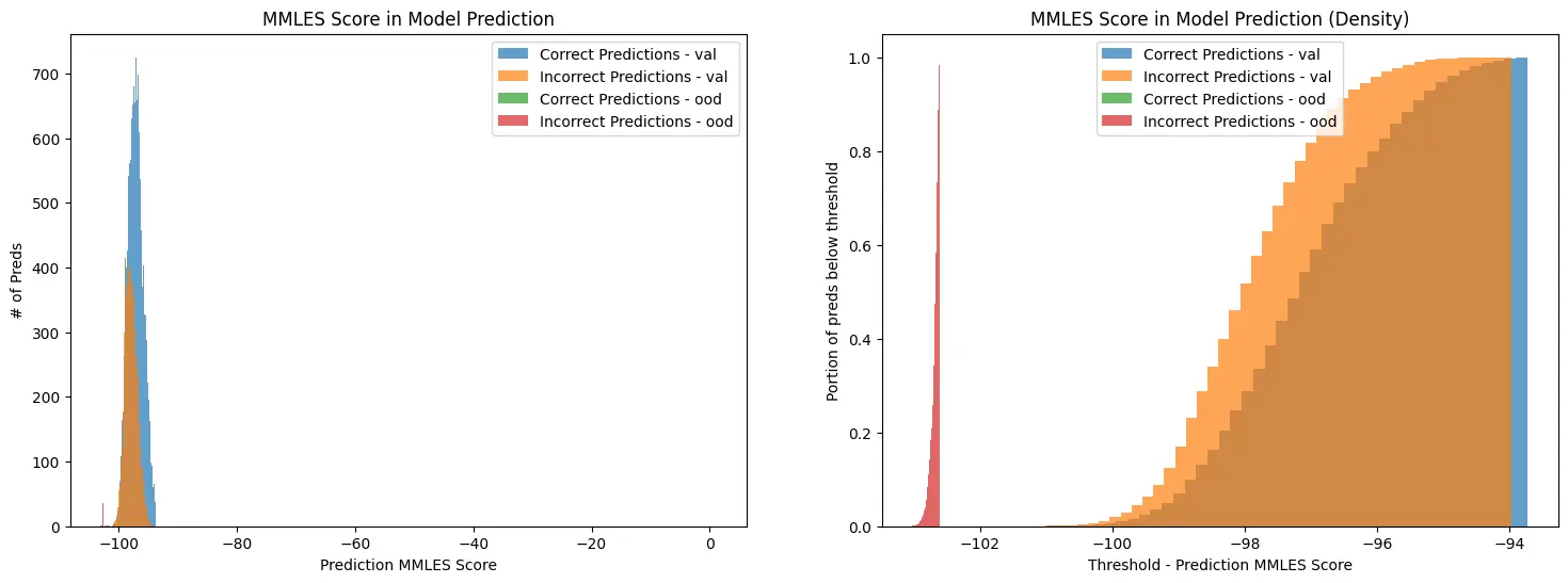
As you can see, from the exact same logits the MMLE scores provide a much stronger delineation of “In-Distribution” vs “Out-of-Distribution” data.

To demonstrate more programmatic use, here is an example of calculating thresholds from the validation data:

val_scores = ... # MMLE scores for the validation samples
mmle_score_thresholds = {
    str(p): np.percentile(val_scores, p)
    for p in [0, 0.05, 0.1, 0.25, 0.5, 0.75, 0.9, 0.95, 1.0]
} # {'0': -102.35904790566515, '0.05': -101.01156283044743, '0.1': -100.71284565474099, '0.25': -100.33496655987776, '0.5': -100.13457710062065, '0.75': -100.00017678930712, '0.9': -99.95630884123959, '0.95': -99.93938238309974, '1.0': -99.92696776594504}

val_scores = ... # MMLE scores for the validation samples
ood_scores = ... # MMLE scores for the OOD samples
for p, t in mmle_score_thresholds.items():
    ood_flagged_as_ood = ood_scores < t
    ood_flagged_as_ood_perc = 100 * ood_flagged_as_ood.sum() / ood_flagged_as_ood.shape[0]
    id_flagged_as_ood = val_scores < t
    id_flagged_as_ood_perc = 100 * id_flagged_as_ood.sum() / id_flagged_as_ood.shape[0]
    print(50*"=")
    print(f"Using p={p}, thresh={t:.2f}")
    print(f"\t{id_flagged_as_ood_perc:.2f}% of valid (in distribution) samples would be incorrectly flagged as OOD")
    print(f"\t{ood_flagged_as_ood_perc:.2f}% of invalid (out of distribution) samples would be correctly flagged as OOD")

# ==================================================
# Using p=0, thresh=-102.36
# 	0.00% of valid (in distribution) samples would be incorrectly flagged as OOD
# 	100.00% of invalid (out of distribution) samples would be correctly flagged as OOD
# ==================================================
# Using p=0.05, thresh=-101.01
# 	0.05% of valid (in distribution) samples would be incorrectly flagged as OOD
# 	100.00% of invalid (out of distribution) samples would be correctly flagged as OOD
# ==================================================
# Using p=0.1, thresh=-100.71
# 	0.10% of valid (in distribution) samples would be incorrectly flagged as OOD
# 	100.00% of invalid (out of distribution) samples would be correctly flagged as OOD
# ==================================================
# Using p=0.25, thresh=-100.33
# 	0.25% of valid (in distribution) samples would be incorrectly flagged as OOD
# 	100.00% of invalid (out of distribution) samples would be correctly flagged as OOD
# ...

For more details, I’ve upload the full notebook.