Stochastic Gradient Descent + SVM Classifier in R
Dataset
The code snippet presented here was written to deal with a collection of data on adult income hosted by the UC Irvine learning data repository. The dataset can be obtained here: https://archive.ics.uci.edu/ml/datasets/Adult
Stochastic Gradient Descent for SVMs
Naive Bayes classifiers are really just a decision rule that compares two products of posterior probability and cost for getting something wrong. Support Vector Machines skip some of the calculations and jump right to searching for weight values. This search requires choosing weights to minimize the cost of errors during training plus the cost of errors in the future. So, we have a complex cost function (F) and we wish to search for a set of values that will minimize that cost function. One way to search for that minimum is to start our variables at random values and take steps along an intelligent direction that will lead us to the minimum. If we imagine this cost function (F) is differentiable, a Taylor series would indicate that the negative gradient is a good search direction for the minimization of F. So we choose our search direction to be the negative gradient. Only problem is, in many cases there is too much data to compute the gradient of F. This is where stochastic gradient descent comes in.
Because the gradient of F is too complex to compute for high dimensional space with many training examples, we’ll turn to stochastic gradient descent. What we’ll do is randomly pick 1 example at a time of the N total training examples. We’ll compute the gradient of the cost function for that example alone and report that vector as the search direction. The computation of this gradient isn’t too intensive because its only 1 example. We’ll then take a step in that direction of a certain length and repeat the process using a new random training example. The key here is that the EXPECTED VALUE of these individual search directions is actually equal to the gradient of F. This is because each is being pulled from the pool of training examples that would be used to calculate the entire gradient of F. It is unlikely that any are actually the gradient, but over time the steps will average out to the right direction even if certain steps are in the wrong direction.
How far should we step in the computed direction? Well we aren’t positive that the direction is correct, but we know on average the chosen directions will lead us along the gradient. To deal with this early uncertainty but later confidence, we’ll use a series of step lengths that decrease over time. Mathematically this equates to maintaining two properties. 1. The limit of the last step as the number of steps approaches infinity should be zero. And 2. The limit of the summation of all the steps as the number of steps approaches infinity should be infinity. Why do we maintain these properties? Because presumably if you’ve been moving for a while, you are probably going in the right direction. If you haven’t been moving for a while, you might not have accumulated enough average movement in the right direction, so you should take BIG steps in case you need to make up for the accumulated error. The # of steps are divvied up into different groups called epochs, each with a smaller step length. For example, if you had 1000 steps placed into 10 epochs, you would make 100 steps at every one of 10 different step lengths.
Results
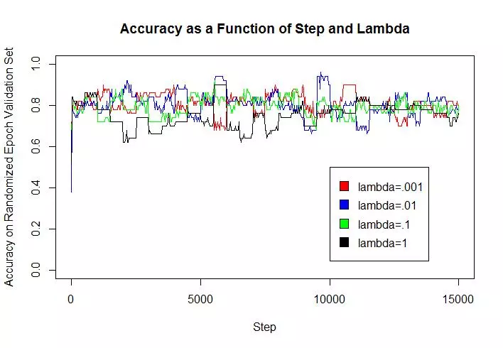
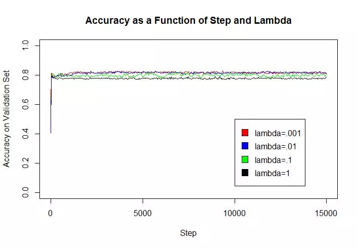
An estimate of the accuracy of the best classifier on the held out (test) data was .814, the mean of 5 different runs on the algorithm. The regularization constant did not seem to greatly affect model accuracy (particularly on the test set) considering the scale at which it varied (factor of 1000). High lambda values (.1 and 1), however, led to loss of accuracy on the validation set, because they allowed for more examples to be misclassified or fall within the margin. Whereas small lambda values could improve accuracy on the training examples but decrease the model’s ability to generalize to new data.
Implementation
The goal here was to write a program from scratch to train a support vector machine on this data using stochastic gradient descent. The final Support Vector Classifier classifies the income bracket (less than or greater than $50k) of an example adult. Only continuous attributes from the dataset were used during training. The program searches for an appropriate value of the regularization constant among a few order of magnitude λ = [1e − 3, 1e − 2, 1e − 1, 1]. A validation set is used for this search. The program uses 100 epochs, each with 500 steps. The step size is constant for each step in a given epoch, but decreases as the epoch increases. In each epoch, the program separate s out 50 training examples at random for evaluation. Accuracy of the current classifier is computed on the set held out for the epoch every 30 steps.
#------------------------------------- SETUP WORK --------------------------------------
#clear the workspace and console
rm(list=ls())
cat("\014") #code to send ctrl+L to the console and therefore clear the screen

#setup working directory
setwd('~/DirectoryNameGoesHere')
#import libraries to help with data splitting/partitioning,
#cross validation and easy classifier construction
library(klaR)
library(caret)
library(stringr)


#------------------------------------- Acquire and Pre-Process Data------------------------------

#read all the data into a single table
allData <- read.csv('adult.txt', header = FALSE)

#grab the labels from the main data file... use as.factor to make
#the format comptabile with future functions to be used
labels <- as.factor(allData[,15])


#grab the features from the main data file, removing the labels
#assume no data is missing... ie: ignore missing values without noting them as NA
allFeatures <- allData[,-c(15)]

#the continous features are in cols 1,3,5,11,12,13
continuousFeatures <- allFeatures[,c(1,3,5,11,12,13)]

#there are no ? (missing feature) for any of the continuous feature, so this modification is irrelevant
#adjust the features such that a 0 is reported as "NA"
#for (f in c(1,2,3,4,5,6))
#{
#  #determine which examples had a 0 for this feature (ie: unknown value)
#  examplesMissingFeatureF <- continuousFeatures[, f] == ?
#  #replace all these missing values with an NA
#  continuousFeatures[examplesMissingFeatureF, f] = NA
#}
#remove any example with an NA
#continuousFeatures[complete.cases(continuousFeatures),]

#normalize the features (mean center and scale so that variance = 1 i.e. convert to z scores):

continuousFeatures<-scale(continuousFeatures)

#convert labels into 1 or -1
labels.n = rep(0,length(labels));
labels.n[labels==" <=50K"] = -1;
labels.n[labels==" >50K"] = 1;
labels = labels.n;
rm(labels.n);


#Separate the resulting dataset randomly
#break off 80% for training examples
trainingData <- createDataPartition(y=labels, p=.8, list=FALSE)
trainingFeatures <- continuousFeatures[trainingData,]
trainingLabels <- labels[trainingData]


#Of the remaining 20%, half become testing exmaples and half become validation examples
remainingLabels <- labels[-trainingData]
remainingFeatures <- continuousFeatures[-trainingData,]

testingData <- createDataPartition(y=remainingLabels, p=.5, list=FALSE)
testingLabels <- remainingLabels[testingData]
testingFeatures <- remainingFeatures[testingData,]

validationLabels <- remainingLabels[-testingData]
validationFeatures <- remainingFeatures[-testingData,]


#------------------------------------- DEFINE AN ACCURACY MEASURE ----------------------------
getAccuracy <- function(a,b,features,labels){
  estFxn = features %*% a + b;
  predictedLabels = rep(0,length(labels));
  predictedLabels [estFxn < 0] = -1 ;
  predictedLabels [estFxn >= 0] = 1 ;

  return(sum(predictedLabels == labels) / length(labels))
}


#------------------------------------- SETUP Classifier --------------------------------------
numEpochs = 100;
numStepsPerEpoch = 500;
nStepsPerPlot = 30;


evalidationSetSize = 50;

c1 = 0.01 #set "a" for determining steplength
c2 = 50 #set "b" for determining steplength
lambda_vals = c(0.001, 0.01, 0.1, 1);
bestAccuracy = 0;
accMat <- matrix(NA, nrow = (numStepsPerEpoch/nStepsPerPlot)*numEpochs+1, ncol = length(lambda_vals)); #vector for storing accuracy for each epoch
accMatv <- matrix(NA, nrow = (numStepsPerEpoch/nStepsPerPlot)*numEpochs+1, ncol = length(lambda_vals)); #accuracy on validation set (not epoch validation set)

for(i in 1:4){
  lambda = lambda_vals[i];
  accMatRow = 1;
  accMatCol = i; #changes with the lambda

  #set a and b to 0 initially:
  a = rep(0,ncol(continuousFeatures));
  b = 0;

  stepIndex = 0;

  for (e in 1:numEpochs){

    #divide into training and validation set for epoch (validation set size = evalidationSetSize -> 50 datapoints):
    etrainingData <- createDataPartition(y=trainingLabels, p=(1 - evalidationSetSize/length(trainingLabels)), list=FALSE)

    etrainingFeatures <- trainingFeatures[etrainingData,]
    etrainingLabels <- trainingLabels[etrainingData]

    evalidationFeatures <- trainingFeatures[-etrainingData,]
    evalidationLabels <- trainingLabels[-etrainingData]

    #set the steplength (eta)
    steplength = 1 / (e*c1 + c2);

    for (step in 1:numStepsPerEpoch){
      stepIndex = stepIndex+1;
      index = sample.int(nrow(etrainingFeatures),1);
      xk = etrainingFeatures[index,];
      yk = etrainingLabels[index];

      costfxn = yk * (a %*% xk + b); #not actually the cost function!

      if(costfxn >= 1){

        a_dir = lambda * a;
        a = a - steplength * a_dir;
        #b = b

      } else {

        a_dir = (lambda * a) - (yk * xk);
        a = a - steplength * a_dir;
        b_dir = -yk
        b = b - (steplength * b_dir);

      }


      #log the accuracy
      if (stepIndex %% nStepsPerPlot == 1){#30){
        accMat[accMatRow,accMatCol] = getAccuracy(a,b,evalidationFeatures,evalidationLabels);
        accMatv[accMatRow,accMatCol] = getAccuracy(a,b,validationFeatures,validationLabels);
        accMatRow = accMatRow + 1;
      }

    }

  }

  tempAccuracy = getAccuracy(a,b,validationFeatures,validationLabels)
  print(str_c("tempAcc = ", tempAccuracy," and bestAcc = ", bestAccuracy) )
  if(tempAccuracy > bestAccuracy){
    bestAccuracy = tempAccuracy
    best_a = a;
    best_b = b;
    best_lambdaIndex = i;
  }

}


getAccuracy(best_a,best_b, testingFeatures, testingLabels)


#Plot the accuracy during training
colors = c("red","blue","green","black");
xaxislabel = "Step";
yaxislabels = c("Accuracy on Randomized Epoch Validation Set","Accuracy on Validation Set");
title="Accuracy as a Function of Step and Lambda";
ylims=c(0,1);

stepValues = seq(1,15000,length=500)

mats =  list(accMat,accMatv);


for(j in 1:length(mats)){

  mat = mats[[j]];

  for(i in 1:4){

   if(i == 1){
     plot(stepValues, mat[1:500,i], type = "l",xlim=c(0, 15000), ylim=ylims,
         col=colors[i],xlab=xaxislabel,ylab=yaxislabels[j],main=title)
    } else{
      lines(stepValues, mat[1:500,i], type = "l",xlim=c(0, 15000), ylim=ylims,
          col=colors[i],xlab=xaxislabel,ylab=yaxislabels[j],main=title)
    }
   Sys.sleep(1);
  }
  legend(x=10000,y=.5,legend=c("lambda=.001","lambda=.01","lambda=.1","lambda=1"),fill=colors);

}


Comments