Parametric Regression via Kernel Smoothing
Dataset
The data used here is comprised of temperature measurements from 112 weather stations in Oregon. The station positions are provided in multiple units, but UTM units were used for this analysis.
The dataset is located here: http://www.geos.ed.ac.uk/homes/s0198247/Data.html
Goals
Github repo available here: https://github.com/dcyoung/Regression-Kernel-Smoothing
The code performs regression of spatial data using kernel functions…
- Uses kernel functions to build various linear regressions predicting the annual mean of the minimum temperature as a function of position.
- Predicts and plots the average annual temperature at each point on a 100x100 grid spanning the weather stations.
- Investigates a regularized kernel method using the lasso.
- Investigates the effect of different choices of elastic net constant (alpha)
- UnRegularized Parametric Regression
Cross Validation Code: https://github.com/dcyoung/Regression-Kernel-Smoothing/blob/master/src/FindOptimalScale.R
Plotting Code: https://github.com/dcyoung/Regression-Kernel-Smoothing/blob/master/src/UnregularizedRegression.R
A kernel method was used to smooth the data with a gaussian kernel function. Note: Smoothing was performed on a processed data set which was obtained by averaging the reported T_min at each location over all times (i.e one interpolate). Each data point was used as a base point, and the search was performed over a range of six scales. For each scale an 8 fold cross validation was performed and a mean MSE value was recorded. For each fold, the annual mean min temperature was predicted at each point on a 100x100 evenly spaced grid spanning the subset of weather stations comprising the training set for the fold. Predictions for the fold’s test set were generated using the built model and the values were compared to the actual min temperature of the validation stations. The difference was recorded as MSE and the best scale was chosen as the scale which yielded the smallest average MSE across 8 folds.
| Scale | Average MSE across 8 folds |
|---|---|
| 31684.73 | 252.067 |
| 63369.46 | 8.028208 |
| 126738.9 | 6.474178 |
| 190108.4 | 6.67963 |
| 253477.9 | 6.656381 |
| 380216.8 | 6.805604 |
The scales corresponded to multiples of the average distance between stations. The multiples were 0.25, 0.5, 1, 1.5, 2, and 3. Of all the compared scales, the final scale was chosen as h= 126738.9 which was also the average distance between points. This scale was chosen as it yielded the smallest average cross validated MSE. The MSE appeared much worse for scales that were too small, and only slightly worse for scales that were proportionally too big. This is most likely because once a scale threshold is reached, the model is decent but continuing to increase the scale can lead to over-fitting of sorts.
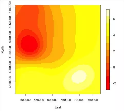
Once the scale was selected, all of the stations were used as a training set to generate a model at that scale. Min temperatures for an even 100x100 grid were then predicted using this model and plotted as an image.

Lasso Regularization
Source code here: https://github.com/dcyoung/Regression-Kernel-Smoothing/blob/master/src/RegularizedRegression.R The same kernel method from the unregularized regression was regularized using the lasso, and again predictions were generated to find the mean annual min temperature at each point on the same 100x100 grid. The regularization constant was chosen using cross validation (cv.glmnet did all the work). Again, a range of 6 scales were used and here the lasso regression effectively pruned unnecessary scales with its internal cross validation and ability to cut out features. Again the predictions were plotted as an image.
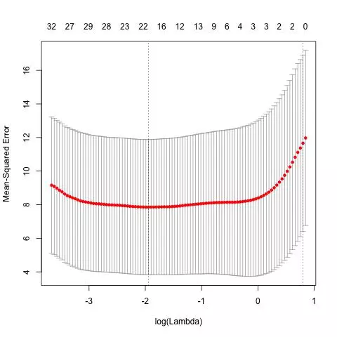
The final number of predictors used by the model was 14. The MSE appears parabolic around the optimal number of predictors which was 14. The error grows faster as the number of predictors decreases from 14, compared to its growth rate as the number of predictors increases from 14. The log of the optimal regularization constant can be read off the graph below and is roughly 1.6.
Experimenting with different values for Elastic Net constant (alpha)
The regularized regression was repeated but with varying ‘alpha’. The effect of different choices of elastic net constant (alpha) was investigated using 3 different alpha values (0.25, 0.5, 0.75). As alpha increases, the regularization constant (lambda) decreased. See the table below.
| Alpha | Regularization Constant (Lambda) |
|---|---|
| 0 | 25.60592 |
| 0.25 | 0.87035 |
| 0.5 | 0.29995 |
| 0.75 | 0.20949 |
| 1 | 0.14315 |
Looking at the heatmaps, at alpha =0, the heatmap is clearly more blurred. At alpha = 0.25 and above, the images look more similar to one another except that alpha = 0.25 is missing a small valley. The least spatial blurring appears to be at alpha = 1.



Comments