Photometric Stereo: Shape from Shading
Overview

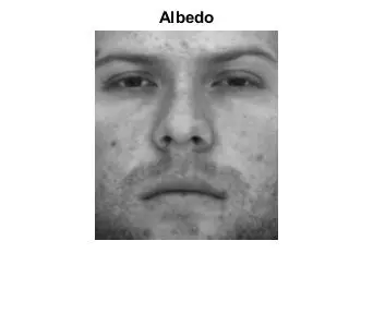
The goal here was to implement shape from shading as described in Forsyth & Ponce 2nd Edition, in order to reconstruct albedo and shape in the form of surface height-maps. The technique was applied to images of faces.
The simple photometric stereo implemented here assumes the following:
- A lambertian object
- A local shading model (each point on a surface receives light only from sources visible at that point… ie: no global illumination)
- A set of known light source directions
- A set of pictures of an object, obtained in exactly the same camera/object configuration but using different light sources
- Orthographic projection
Implementation
The project goal is to reconstruct the surface as a heightmap above the x-y plane. This is accomplished through the intermediate step of recovering surface normals and using those normals to recover the surface heights. Images of subjects from from the Yale Face database were used for testing. For each subject the following was performed:
- Images and light source directions were acquired for 64 different light source directions + an ambient image
- The data was pre-processed, which involved subtracting the ambient image from each image in the light source stack and normalizing the intensities
- The albedo and surface normals were estimated, using a least squares solution of constructed linear systems
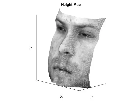
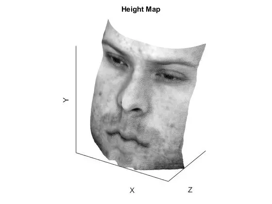
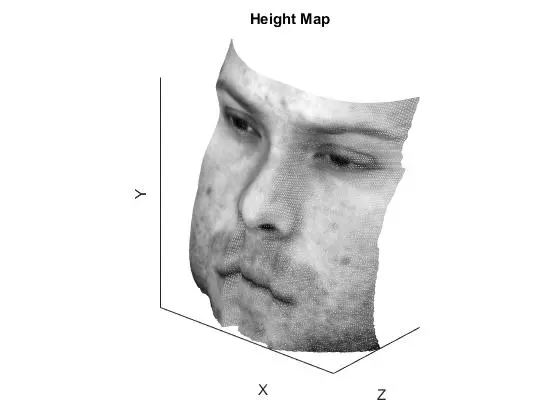
- A surface height map was computed by integration. Multiple different paths were computed to compare the results.
Main Script
%clear everything
clear all;
clc;

% path to the folder and subfolder
root_path = 'C:/DirectoryNameGoesHere';
subject_name = 'yaleB01';

%'average'; % 'column', 'row', 'average', 'random'
integration_method = 'average';


%% load images
full_path = sprintf('%s%s/', root_path, subject_name);
[ambient_image, imarray, light_dirs] = LoadFaceImages(full_path, subject_name, 64);
image_size = size(ambient_image);


%% preprocess the data:
%% subtract ambient_image from each image in imarray
%% make sure no pixel is less than zero
%% rescale values in imarray to be between 0 and 1
pre_processed_imarray = zeros(size(imarray));
for i = 1 : size(imarray,3)
   pre_processed_imarray(:,:,i) = PreProcessImage(imarray(:,:,i), ambient_image);
end
imarray = pre_processed_imarray;


%% get albedo and surface normals (you need to fill in photometric_stereo)
[albedo_image, surface_normals] = photometric_stereo(imarray, light_dirs);

%% reconstruct height map (you need to fill in get_surface for different integration methods)
height_map = get_surface(surface_normals, image_size, integration_method);


%% display albedo and surface
display_output(albedo_image, height_map);

%% plot surface normal
plot_surface_normals(surface_normals);
Pre-Processing
Pre-processing is very straight forward. Normalizing every pixel between 0 and 255 (max possible intensity) ensures consistency.
function [ output ] = PreProcessImage( targetImg, ambientImg )
%subtract the ambient image from the light source stack image, set
%any negative values to zero, rescale the resulting intensities to between
%0 and 1 (they are originally between 0 and 255)
    output = targetImg - ambientImg;
    indices = output<0;
    output(indices) = 0;
    output = output./255;
end
Calculating Albedo and Surface Normals
Having obtained the source vectors and intensity values, the basis of the problem can be laid out as follows:
- Known: source vectors Sj and pixel values Ij(x,y)
- Unknown: surface normal N(x,y) and albedo p(x,y)
Assuming the response function of the camera is a linear scaling by a factor of “k”, Lambert’s law and a bit of regrouping terms will yield:
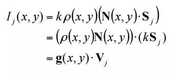
where g(x,y) refers to the normals scaled by albedo and Vj refers to the scaled light source vector.
A linear system can be setup for each pixel according to this formula. This system can then be solved for the normals and alebdo. Stacking all the linear systems on top of one another in matrices will yield the following:
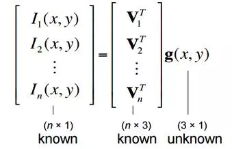
Obtaining a least-squares solution for g(x,y) is simple in Matlab. Recall that g(x,y) must be equal to N(x,y)*p(x,y) and since N(x,y) is a unit normal, the albedo p(x,y) is given by the magnitude of g(x,y).
function [albedo_image, surface_normals] = photometric_stereo(imarray, light_dirs)
% imarray: h x w x Nimages array of Nimages no. of images
% light_dirs: Nimages x 3 array of light source directions
% albedo_image: h x w image
% surface_normals: h x w x 3 array of unit surface normals


    %grab the dimensions
    [h,w,numImages] = size(imarray);
    %initialize the
    albedo_image = zeros(h,w);
    surface_normals = zeros(h,w,3);

    linear_system = zeros(numImages,1);
    g = zeros(3,1);
    for col = 1:w
        for row = 1:h
            linear_system(1:numImages,1) = imarray(row,col,1:numImages);
            g = light_dirs\linear_system;
            magnitude = norm(g);
            albedo_image(row,col) = magnitude;
            surface_normals(row, col, :) = g./magnitude;
        end
    end

end
Compute Surface Height Map by Integration
Here the surface height map is computed via integration. Instead of continuous integration of the partial derivatives over a path, different strategies are compared which simply sum the discrete values/steps that make up the path. In the “average” case, the integration is performed over both the row and column first paths, and then averaged. In the random case, 100 random paths starting from pixel 1,1 are used as the paths for integration. For each, a random increment of row or column creeps the integration closer to the target pixel location. This was easy to implement, and yields descent results when the average is taken, but it is limited. An improved implementation may have started the integration from different pixels values (such as different corners) so that the error did not accumulate towards one far corner. To keep the code simple, the built in Matlab function “cumsum” is used to perform the cumulative summations for the integrations. The partial derivatives are calculated and stored in matrices before the integrations are performed in order to speed things up. Even the 100 integration paths for the random case are performed in just a few seconds.
function  height_map = get_surface(surface_normals, image_size, method)
% surface_normals: 3 x num_pixels array of unit surface normals
% image_size: [h, w] of output height map/image
% height_map: height map of object

    h = image_size(1);
    w = image_size(2);
    height_map = zeros(h,w);

    dfdx = surface_normals(:,:,1)./surface_normals(:,:,3);
    dfdy = surface_normals(:,:,2)./surface_normals(:,:,3);

    for u = 1:h
        for v = 1:w
            switch method
                case 'column'
                        col_sum = cumsum(dfdy(1:u, 1),1); %col
                        row_sum = cumsum(dfdx(u, 1:v),2); %row
                        height_map(u,v) = col_sum(length(col_sum)) + row_sum(length(row_sum));
                case 'row'
                        row_sum = cumsum(dfdx(1, 1:v),2); %row
                        col_sum = cumsum(dfdy(1:u, v),1); %col
                        height_map(u,v) = row_sum(length(row_sum)) + col_sum(length(col_sum));
                case 'average'
                        z = zeros(1,2);
                        col_sum = cumsum(dfdy(1:u, 1),1); %col
                        row_sum = cumsum(dfdx(u, 1:v),2); %row
                        z(1) = col_sum(length(col_sum)) + row_sum(length(row_sum));

                        row_sum = cumsum(dfdx(1, 1:v),2); %row
                        col_sum = cumsum(dfdy(1:u, v),1); %col
                        z(2) = row_sum(length(row_sum)) + col_sum(length(col_sum));
                        height_map(u,v) = mean(z);
                case 'random'
                        numRandPaths = 100;
                        height_maps = zeros(h,w,numRandPaths);
                        for i = 1:numRandPaths
                            row_sum = 0;
                            col_sum = 0;
                            r = 1;
                            c = 1;
                            while r < u && c < v
                                if rand > 0.5
                                    row_sum = row_sum + dfdx(r,c);
                                    c = c + 1;
                                else
                                    col_sum = col_sum + dfdy(r,c);
                                    r = r + 1;
                                end
                            end
                            while r < u
                                col_sum = col_sum + dfdy(r,c);
                                r = r + 1;
                            end
                            while c < v
                                row_sum = row_sum + dfdx(r,c);
                                c = c + 1;
                            end
                            height_maps(u,v,i) = row_sum + col_sum;
                        end
                        %height_map(u,v) = row_sum + col_sum;
                        height_map(u,v) = mean(height_maps(u,v,:));
                otherwise
                    error('Specified method is invalid.');
            end
        end
    end
end
Results
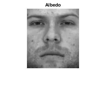
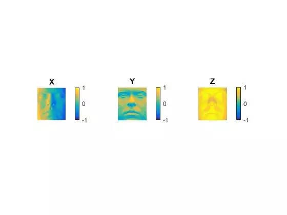
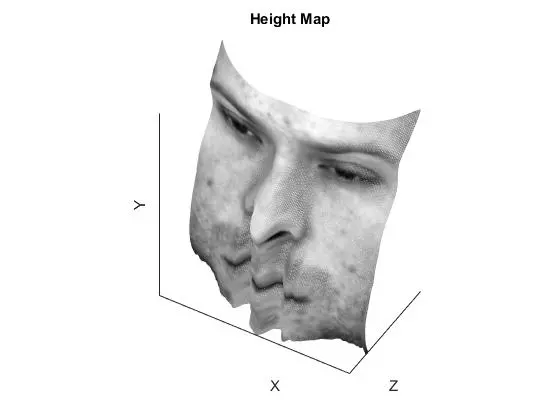
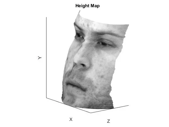
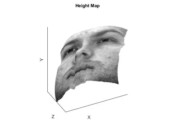
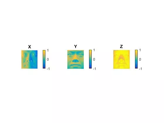
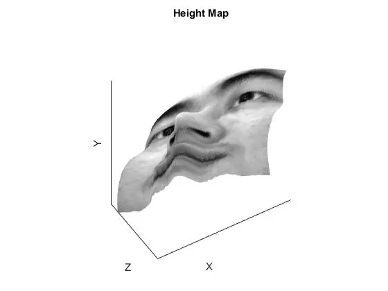
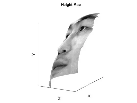
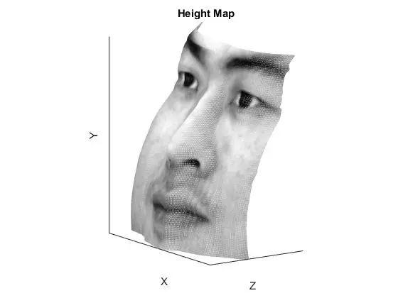
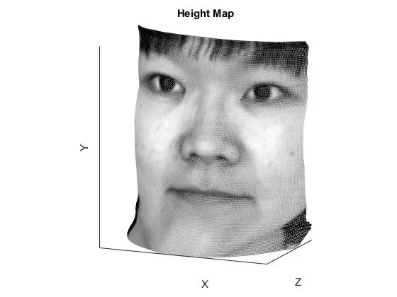
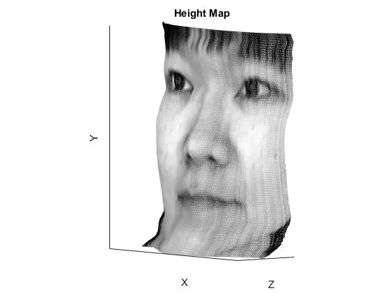
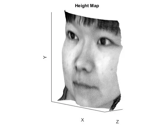
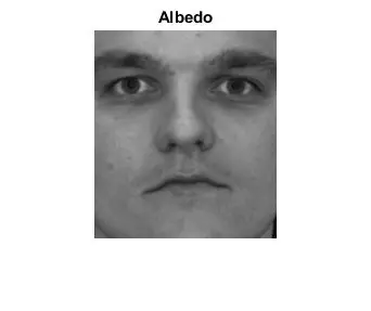
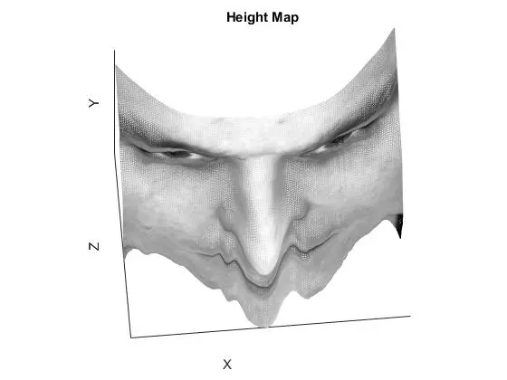
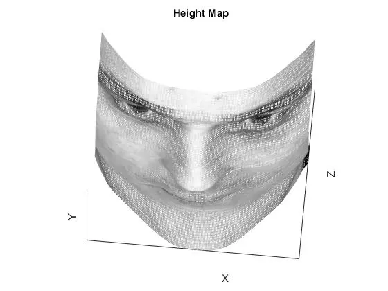
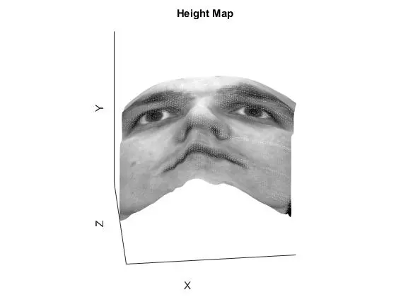
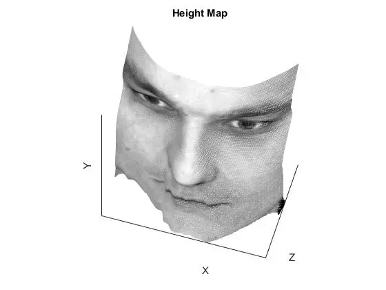
Results were generated for four different faces from the dataset. For each, the following are included:
- calculated albedo
- calculated surface normals
- results of each integration path method, including “row”, “columns”, “average” and “random”
The angles for each photo result were chosen to highlight any unique flaws from that integration path.
YaleB01

YaleB02
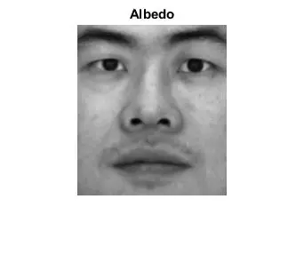
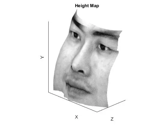
YaleB05
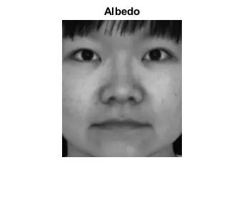
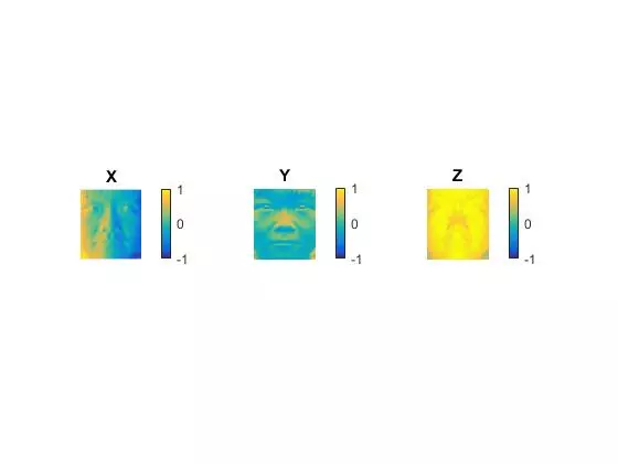
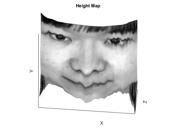
YaleB07

Results Discussion
The row and column integration methods are essentially the same, just operating on different order of axis. The result is an obvious error along one of the axis, but decent results along the other. Averaging the two normally yields superior performance, as it reduces noise from the inferior axis of each. Random integration performs well but accumulates noise in the lower left corner because all integration paths are starting in the top left pixel. A better implementation would have varied the starting pixel for integration and adjusted the integration to be consistent. Increasing the number of paths used for the random average results in better surface accuracy but at the cost of computation time. The best method for all faces was either “average” or “random” depending on the face. If there was a particularly large ripple in one of the faces (such as the row integration of YaleB01), then the random integration performed better than the average integration.
Integration Run-Times Compared
The following table shows the running time of the “get_surface.m” function which performs the integration. The values in each row of the table should all be the same, as the integration method is unchanged and the image size is constant between all faces. The row and columns are very similar in performs save for a miniature difference attributable to additional calculations for transposing the vectors for cumsum. The average is a little more than double the row or column, which makes since as it performs both and then computes their average. Lastly, the random integration method performs 100 trials each with similar cost to rows or columns integration. As expected, the duration is around 100x that of the row or column. This means performance is scaling very well, and fewer trials would lead to a shorter run time.

Violations/Limitations
Recall that the simple photometric stereo implemented here assumes the following:
- A lambertian object
- A local shading model (no global illumination)
- A set of known light source directions
- A set of pictures of an object, obtained in exactly the same camera/object configuration but using different light sources
- Orthographic projection
However, in reality a lot of the previously listed assumptions do not hold true. Contradicting each assumption individually:
- Human skin is far from lambertian. Light can be sub-scattered beneath the skin. Additionally, oil on the skin often makes for an extremely specular surface. This is especially true on the nose, cheeks and chin. Eyes are also extremely specular.
- There is no way for a local shading model to exist in reality. Light will bounce and reflect off surfaces, illuminating surfaces nearby. Inevitably, when light hits a spot on the face it will also contribute to illumination of nearby skin.
- The set of light source directions is known, but there could be imprecision or measurement errors.
- The pictures were hopefully obtained using the same camera/object configuration, but this cannot be verified.
- True Othographic projection is not impossible with the kind of camera used to capture these photos. A rendering program would have to output such images if orthographic view is necessary.
Despite these overwhelming contradictions, the results show that valuable reconstruction of an informative surface can be obtained using shape from shading.
Removing images that seem to violate the assumptions might help the overall performance. Six images appeared to have high specular reflection, and were removed from the dataset (originally 64 images -> now 58 images). The results of this subset of viewpoints are shown below (subset on right, original on left). There did not appear to be any discernible differences.




Comments