Path Planning (Mazes + Pacman)
This writeup summarizes the procedure and results of various path finding algorithms on a grid based maze. It also contains discussion of said results and attempts to provide some insight and reflection on the behavior of each algorithm. The assignment was completed for course CS440 Artificial Intelligence at University of Illinois Urbana Champaign.
Overview of Source
The following source files were written from scratch:
- FileReader.java - Reads the mazes from .txt files and stores them in an array with an intermediate encoding.
- MazeState.java - Reads the intermediate array into a structure that stores the state of the maze and its associated components.
- TreeNode.java - A grid space in the maze in the format of a node with associated properties useful for the search algorithms.
- Search.java - A collection of search algorithms to solve a maze provided a mazestate, also contains the main method used for testing.
- DrawingBoard.java - A class used to draw and animate the state of the maze under various conditions.
The following 2d graphics library was taken from an introductory princeton CS course (http://www.cs.princeton.edu/introcs):
- StdDraw.java - Standard Graphics Library for drawing 2d primitives in java
Maze Format
Mazes are provided in a specific layout via .txt files where ‘%’ stands for walls, ‘P’ for the starting position, and ‘.’ for the goal. The files are modified so the first line holds the dimensions of the maze like so:
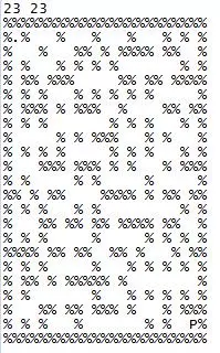
The .txt file is then read into an array and from that array, a custom structure is formed to assist in the path finding by holding the state of the maze. Various search algorithms were implemented and a basic 2D graphics library was used for visual debugging and the creation of path finding animations. The implemented search algorithms include: Depth First Search, Breadth First Search, Greedy and A*. Each of the 4 algorithms was run on 3 different mazes (MediumMaze, BigMaze and OpenMaze). After each run, two values were noted: the number of total path nodes in the final solution as well as the total number of nodes expanded during the algorithm’s run time. Note that these numbers should include the effects of the start and goal nodes.
Implementation
- Breadth first search (which maintains a frontier of equidistant nodes from the origin) was implemented using a queue data structure which made it easy to visit un-visited child nodes before diving deeper.
- Depth first search was implemented using a stack structure and dove into the tree until a root had no more children.
- Greedy search was similar to A* in that it made decisions based off an estimated cost for every node, however the Greedy search only considered the manhattan distance from a node to the goal, and not the accumulated cost of arriving at the node.
- A* search maintains a frontier of nodes at equal path costs, considering both the cost to arrive at the node and the estimated cost to reach the goal. A* was implemented using Manhattan distance as a heuristic, maintaining a set of un-evaluated nodes sorted by total cost (FCost = GCost+HCost, where GCost = path cost to node so far, HCost = manhattan distance). Each loop through the algorithm, the node in the un-evaluated set with the lowest FCost is evaluated and all of its neighboring nodes are checked for previous evaluation, or at least a shorter path if already visited.
The results of the 4 algorithms are shown below:

Medium Maze Solutions
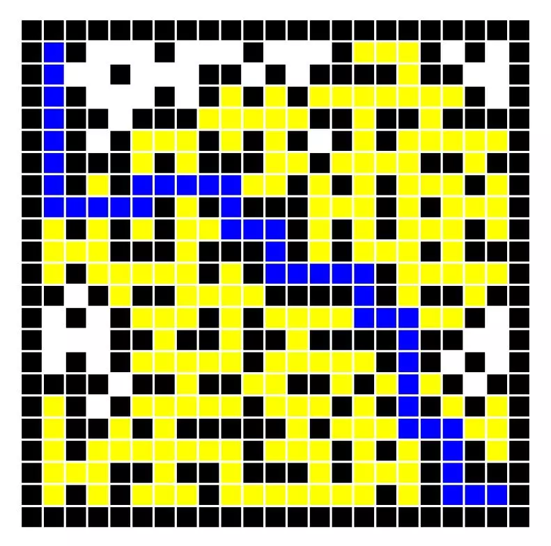
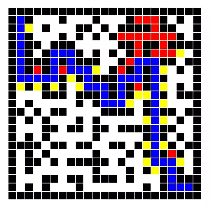
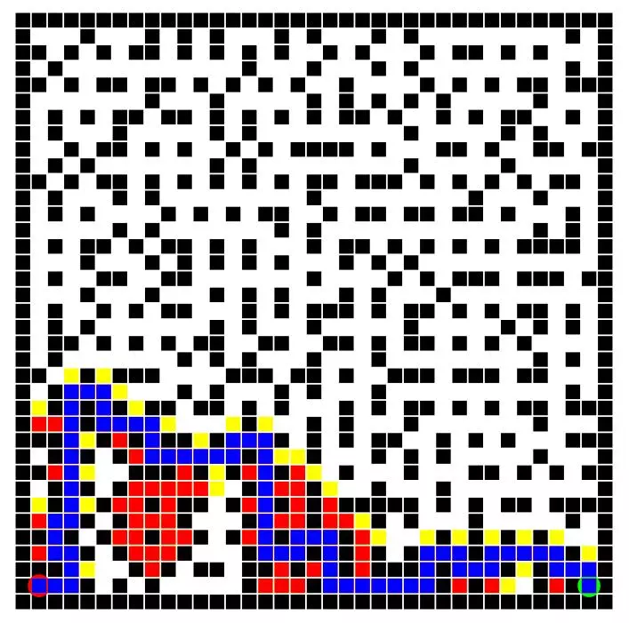
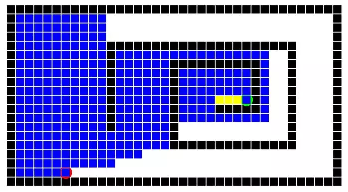
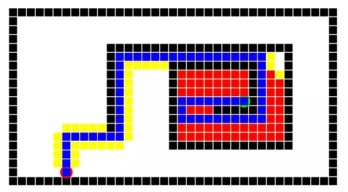
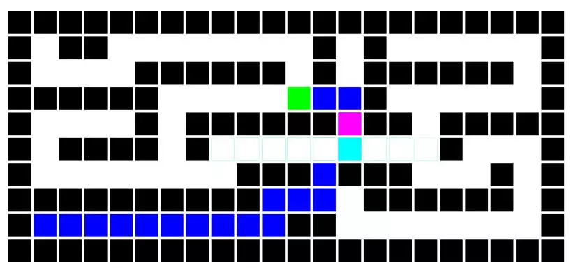
The following 4 images show the solutions to the medium maze using all 4 search algorithms and a unit step cost of 1. The maze is set to only allow horizontal or vertical movement (ie: no diagonal movement). The results of some of these algorithms will vary between implementations due to the order of node consideration on the frontier as well as different solutions to tie breakers. The depth first search is a perfect example of this, where different implementations might say to always fork left at a tie instead of right. For any given maze a certain implementation might get lucky and choose a good node to dive into. Depth first search and greedy search are only guaranteed to return a solution, and not necessarily the optimal solution.Whereas breadth first search and A* will return the optimal solution or one of the optimal solutions if multiple exist. The number of nodes expanded can still vary slightly, depending on tie breakers. The depth first search was surprisingly lucky and the greedy search benefited from the maze having a fairly traversable diagonal. Breadth first search of course visited a lot of nodes, and A* definitely cut down the visitation with the same optimal result. Results are ordered left to right in the following order: DFS, BFS, Greedy, A*.
Big Maze Solutions
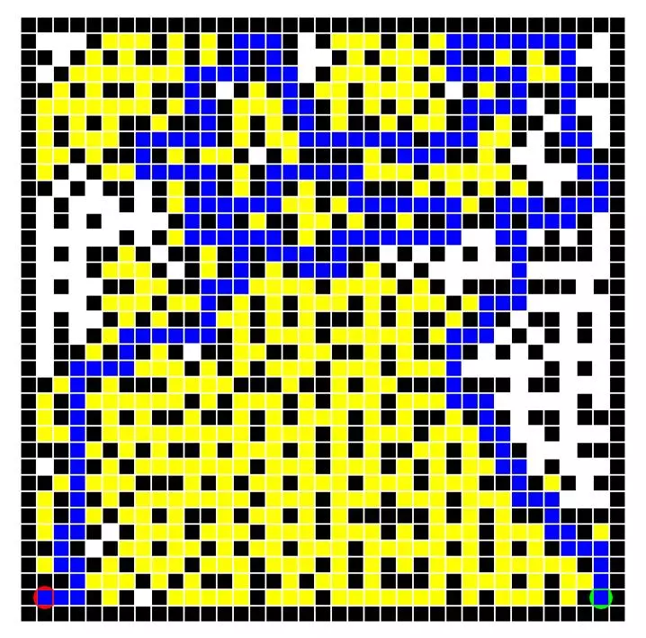
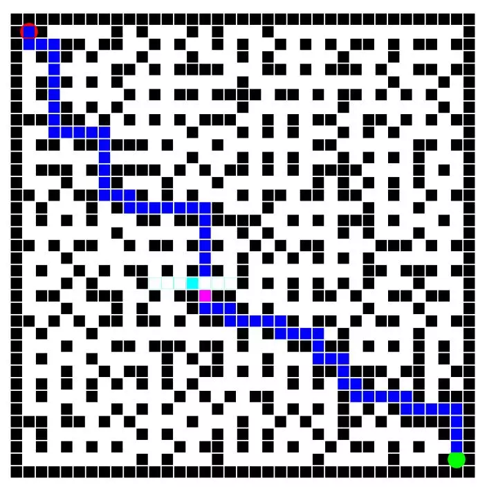
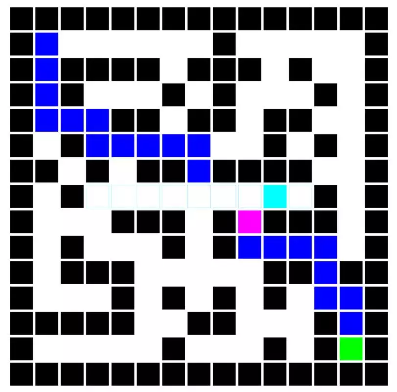
Here depth first search was not as lucky, but greedy was extremely lucky. The breadth first search nearly visited the entire maze, while A* worked a happy medium. Order left to right: DFS, BFS, Greedy, A*.
| DFS | BFS | Greedy | A* |
|---|---|---|---|
Open Maze Solutions
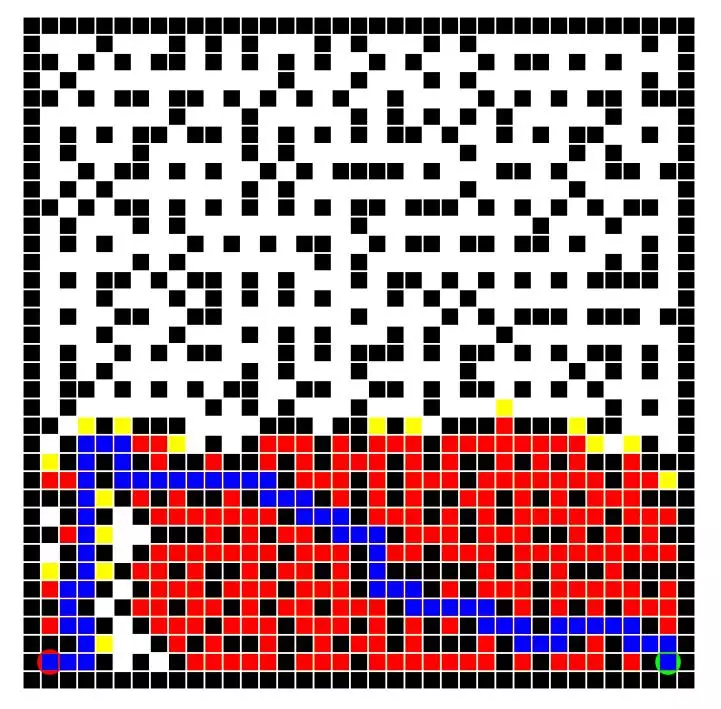
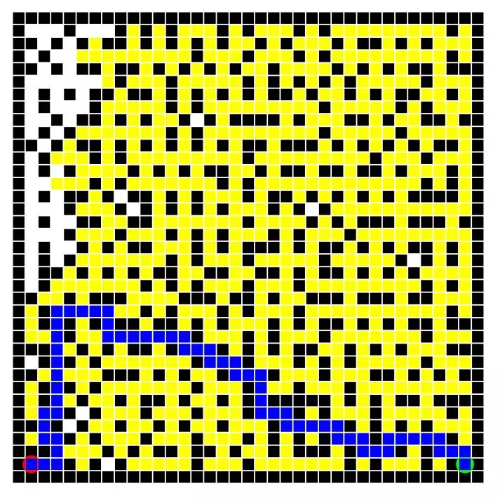
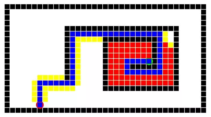
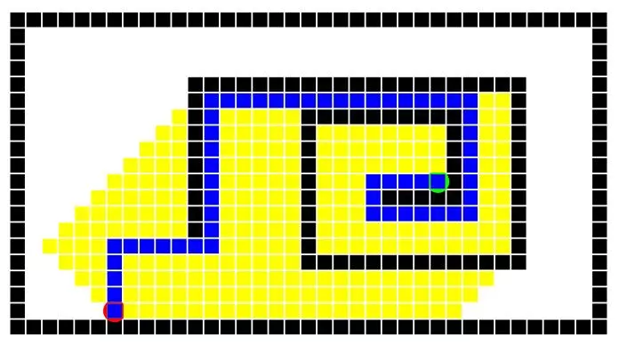
The open maze puzzles demonstrated the characteristics of each algorithm quite overtly. The depth first search was miserably inefficient. The breadth first search explored nodes at an expanding but even radius from the origin which is visible from image. Greedy search fared well once it broke free of the spiral, but it clearly attempted to move towards the goal (disregarding the wall) right off the bat. The A* had to fill most of the spiral as it evenly spread out, but once it broke the spiral, it was as efficient as the greedy and didn’t waste the same cost of exploration that breadth first search did. Order left to right: DFS, BFS, Greedy, A*.
| DFS | BFS | Greedy | A* |
|---|---|---|---|
Penalizing Turns
Next, a modified version of the A* search algorithm was created to take into account the cost of turns. Each cycle the “entity” could move forward or rotate in place. Both actions carried a weight. Looking at any move (forward, backward, leftward or rightward) as a combination of rotations and forward movement, a simple weight function could be applied to different movements without having to actually simulate the rotation. Anytime a neighboring node was considered, the orientation of the last move and the current move were determined and used to calculate the total move cost like so:
int lastMove = FindOrientation(current, current.getParent());
int thisMove = FindOrientation(neighbor, current);
int turnCost = CalculateMoveCost(thisMove, lastMove, forwardCost, rotateCost);
Then the Ghost was set according to the turn cost. Here “turnCost” refers the the cost of move to a neighboring node, not the cost of rotation which is “rotateCost”. This special cost was also used to compare the path cost to to see if an already visited node should be updated.
Results
A* was run on 2 different mazes (small and big) for the following two cases:
- forward movement has cost 2 and any turn has cost 1;
- forward movement has cost 1 and any turn has cost 2.
using two different heuristics (manhattan + another). For the purpose of exploration I ran the algorithm on 6 different cases of Forward and Turn Cost: (2+1, 1+2, 2+2, 2+4, 2+10, 2+15). The values were chosen to see how well the heuristics would react to the increased weight placed on turns. The following results were obtained.
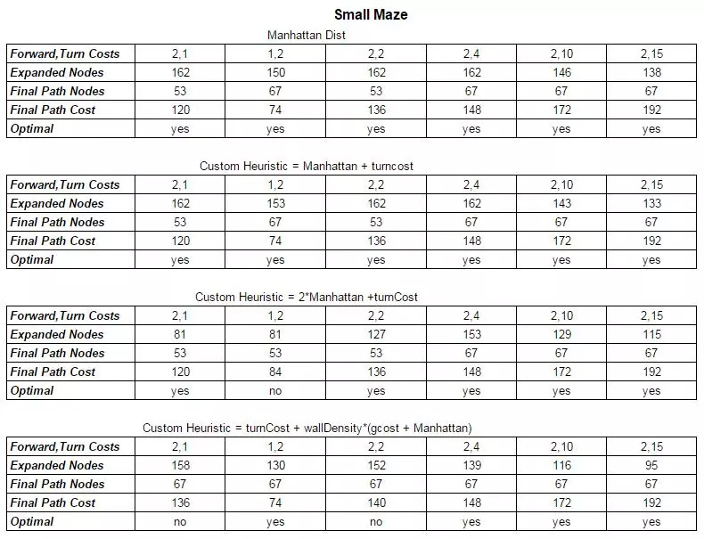
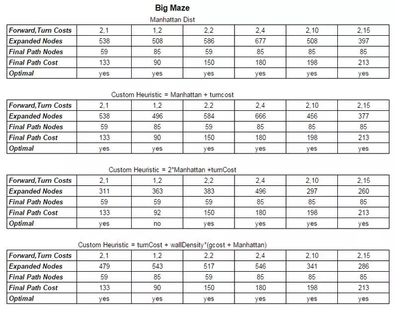
Looking at the small maze it is clear that going from (Forward Cost, Turn Cost) = (F, T) of (2,1) to (1,2) altered the final maze solution. The optimal solution is calculated according to path cost, and with the extra weight on turns, the optimal solution switched from a path of length 53 nodes to a path of length 67 nodes because the total path cost was shorter. Manhattan distance works well as a heuristic and will always provide optimal results but the efficiency can be improved upon. Considering the addition of turn cost into the heuristic demonstrates a heuristic that also guarantees optimal results but with a slight boost in efficiency especially at larger weights on turns. This is expected because it will take into consideration the effect of turns in the HCost of the node and therefore the FCost of the node used extensively in the algorithm. Since turns are impactful here, noting them in the heuristic is useful. But the results aren’t as noticeable at lower turn costs because the manhattan distance simply outweighs the turn cost.
Looking at a custom heuristic of 2*ManhattanDistance + turn cost the results aren’t always optimal, in the case of (1,2), but as the turn cost grows, the enormous increase to efficiency becomes evident. This may not be the best for a reliable metric, but for path finding in games or something where average performance is more of an issue than robustness, this could prove useful.
Lastly I tried to form a complex heuristic that I hoped would prove fruitful, but the results although efficient were not always optimal. The heuristic turnCost + wallDensity(gcost+ManhattanDist) was attempting to incorporate the cost of turns, as well as the density of maze walls in the area between the current node and the goal. The thought was to weight the manhattan distance and the gcost (representing the total fcost) by the wall density (inherently normalized) of the area to be traversed. The efficiency under high turn weights was apparent, but the optimality at lower turn weights wasn’t.
Pacman with a Ghost
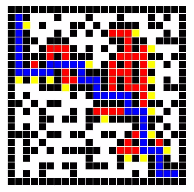
Lastly, a few mazes with ghosts were attempted using a modified A* algorithm under the conditions of unit step cost. The idea was to probe the location of the ghost and predict collisions. Since the ghosts starting location and movement laws were provided, this was absolutely deterministic. The position of the ghost could be reliably determined at any step through the game. The algorithm was modified to predict collisions based on a cycle count (representing a move in the game). Whenever the pacman attempts to make a move, it determines whether there will be a collision and backtracks if so. If the lowest path cost is still on the previously attempted path it will try again and sneak past the ghost when it passes, successfully avoiding a collision.
Both the normal A* algorithm, as well as the modified ghost avoidance algorithm were run on 3 different mazes (small, medium and big). The final path cost, number of path nodes and number of expanded nodes are shown below:

| small | medium | large |
|---|---|---|
Other Path Planning Algorithms: D*, LPA* and D* Lite
A* is a standard algorithm in path planning for games, but games often have the luxury of observable worlds where the locations of obstacles are known ahead of time. In the world of robotics, the goal may be to navigate a space that is unknown or only partially known. While A* can be used to navigate a partially-known environment, it may be inefficient. To move through a partially known environment, A* will plan an initial path based on known information and then modify or replan the entire path as obstacles are encountered. The reason for this is that once a path is found, all intermediate information calculated during the algorithm’s execution is discarded… except for the path itself. So, if A* is navigating an unknown environment and encounters a new obstacle, it will note the obstacle but forget all previously calculated node info for the path when it restarts. This sacrifices computational efficiency.
An alternate algorithm called D*, keeps this information and calculates some other bits that enable faster re-estimation of paths when new obstacles are encountered. This yields much faster run time when planning a path through an unexplored space dense with obstacles. D* is capable of planning paths through completely unknown or even dynamic (changing) environments efficiently without sacrificing optimality. The algorithm gets its name from being similar to A* (hence the *) but supporting dynamic obstacles (hence the D). On a single path plan, A* and D* run similarly. However, if the graph changes as the agent moves along the path, D* is able to quickly compensate. D* will recalculate the best path from the agent’s current position to the goal faster than running a new A* from the current position to the goal. However, D* is considered overly complex and has been rendered obsolete given more modern variations such as D*-Lite.
LPA* (or incremental A*) is a form of A* that keeps information useful in subsequent searches after minor changes to the graph. Ie: if the agent hasn’t moved from the starting location but the graph has changed, then LPA* can adjust the best path quicker than A*. However this does not yield much benefit if the agent is moving along the path when graph changes occur. For this situation, where a new best path is desired as the agent moves along the initial best path, D*-Lite is most useful. D*-Lite makes use of LPA* to effectively mimic the complex D*. D*-Lite guarantees the same results and runs faster than D*.



Comments