Laplacian Blob Detector
In order to track features across scales, detected features must be invariant to affine transformations. However, many common feature detection algorithms (ex: Harris Corner Detector) are not invariant to scale.
A laplacian blob detector is one method to generate scale invariant features. The basic idea is to convolve an image with a “blob filter” at various scales and identify extrema of filter response in the resulting scale space.
Algorithm Outline
- Generate a Laplacian of Gaussian filter
- Iteratively construct a Laplacian scale space
- Filter the image with a scale-normalized Laplacian at current scale
- Store the square of the Laplacian response for the current scale
- Increase the scale by a factor k
- Perform a 3 dimensional non-maximum suppression in scale space
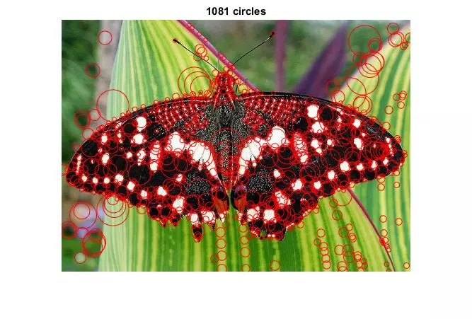
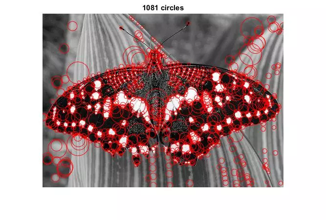
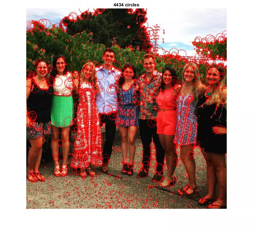
- Display markers for the detected blobs as circles at their characteristic scales
Results
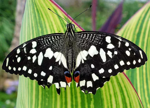
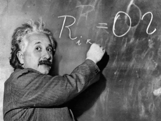
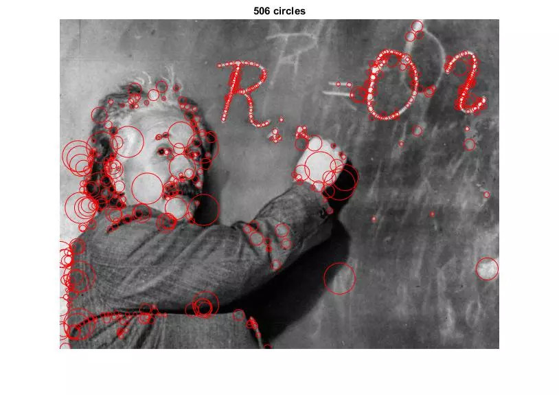
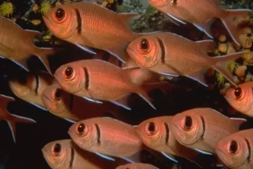
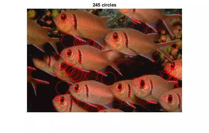
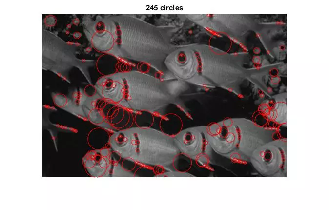
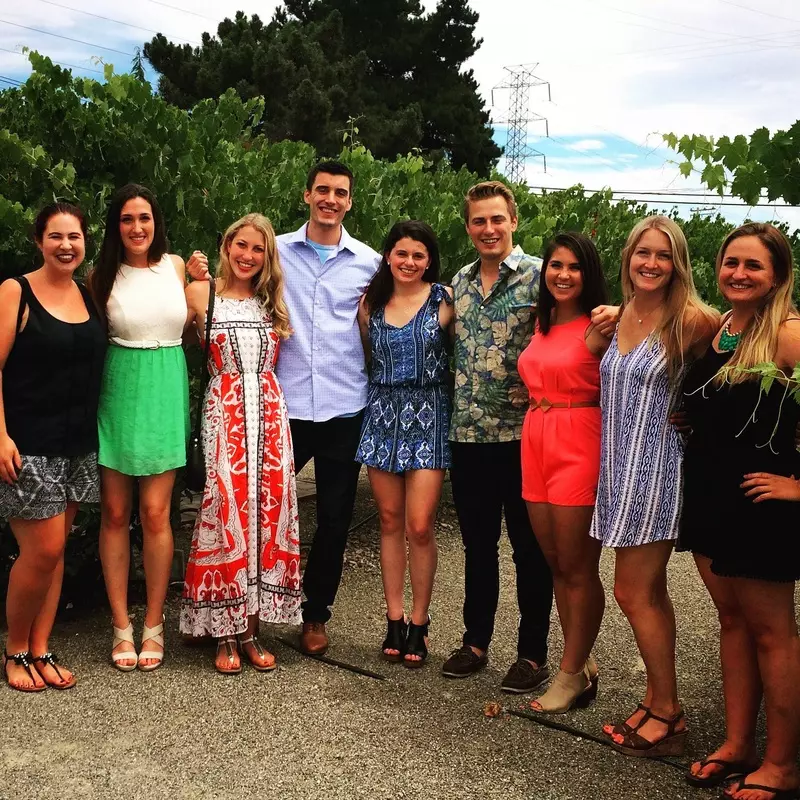
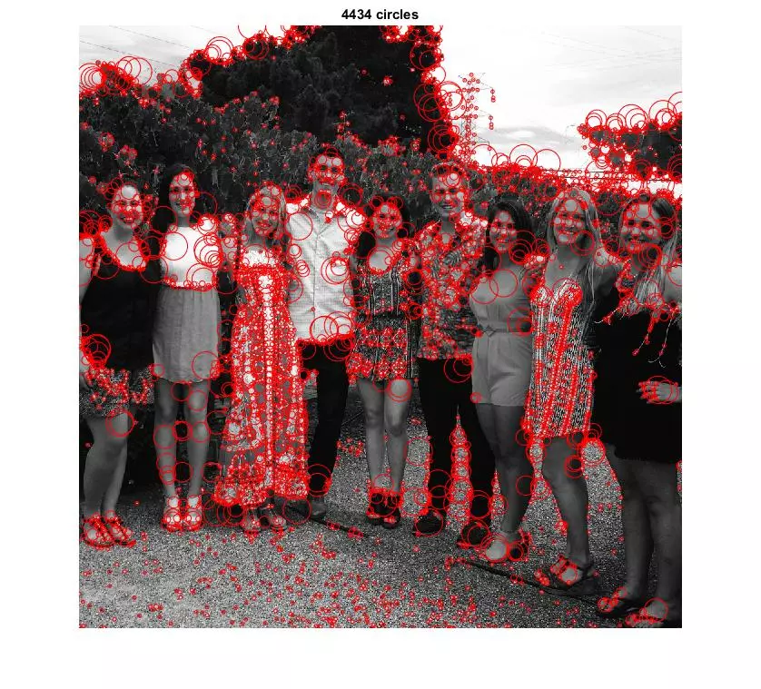
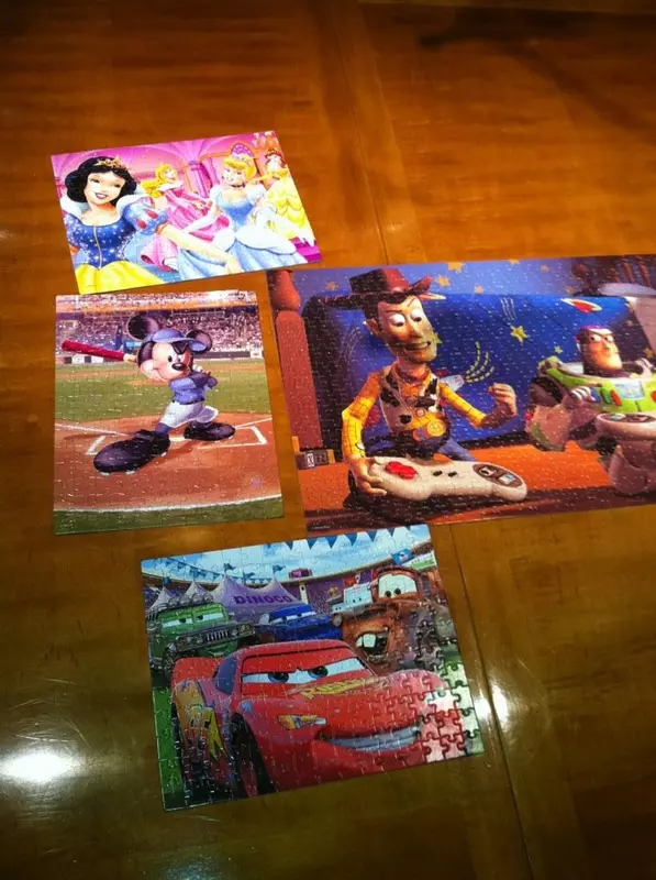
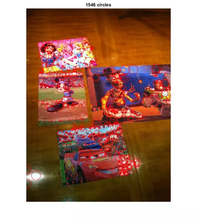
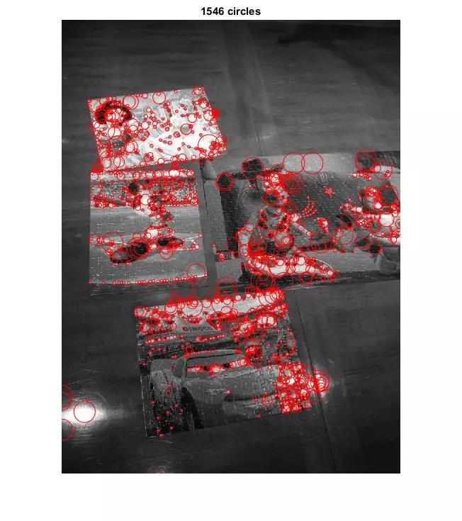
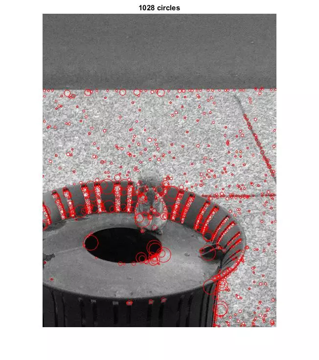
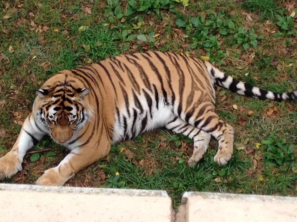
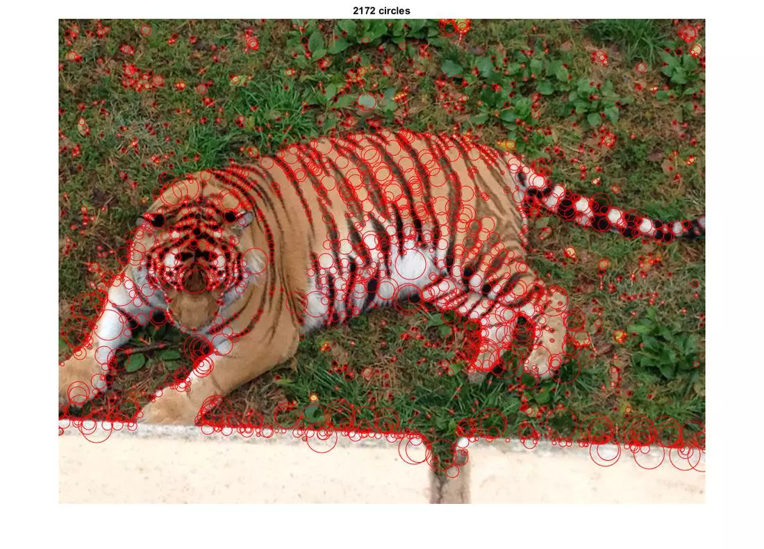
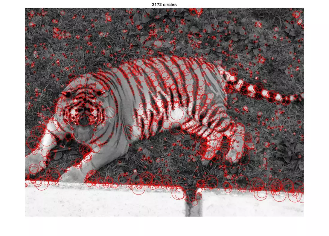
The following results show blobs detected on provided images. The radius of a circle corresponds to the scale of the detected blob.

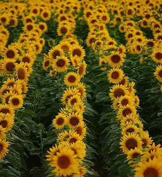
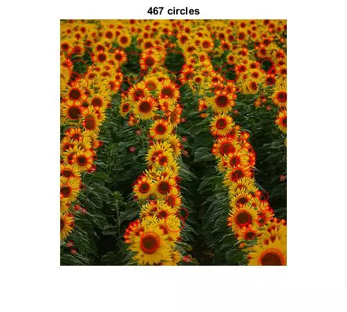
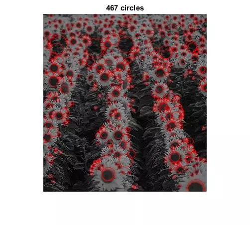
Main Script
This main script provides an example of how to use the written code, as well as some starting parameters. For the important parameters… Sigma was set at 2 (a nice split between 1-3). Later on the kernel size is defined in such a way to guarantee an odd value. The scale multiplier was set at sqrt(sqrt(2)), a number high enough above 1.0 that scales are separated but not so high as to grow too fast. The commented out code under the scale multiplier instantiation shows how the values were printed for each scale during tuning. What I was looking for was a nice spacing such that smaller scaled images would be sampled more often to account for the more rapid shifts from pixel to pixel as compared to sampling the larger scale images less often due to the less rapid changes from pixel to pixel. If the scale multiplier isn’t chosen carefully, and the the kernel size is large relative to the image the resulting scale space will have a few images that are too similar. Lastly, the threshold was tuned to yield a pleasing number of blobs. This was a design choice given the viewed output.
%info for user....
clear all;
clc;

%%%%%%%%%%%%
% Pick image
%%%%%%%%%%%%
%'einstein.jpg'; %'butterfly.jpg'; %'fishes.jpg'; %'sunflowers.jpg';
imgFilename = 'butterfly.jpg';
targetImg = imread(imgFilename);


%%%%%%%%%%%%%%%%%%%%%%%%%%%%%
% Convert image to gray scale
%%%%%%%%%%%%%%%%%%%%%%%%%%%%%

%img_GrayScale = rgb2gray(targetImg);
img_GrayScale = mean(double(targetImg),3)./max(double(targetImg(:)));


%%%%%%%%%%%%%%%%%%%%%%%%%%%%%%%%%%%%%%%%%%%%%%
% Define parameters for desired implementation
%%%%%%%%%%%%%%%%%%%%%%%%%%%%%%%%%%%%%%%%%%%%%%
numScales = 13;
sigma = 2;
scaleMultiplier = sqrt(sqrt(2)); %scale multiplication constant
%for i = 2:numScales
%    1/(scaleMultiplier^(i-1))
%end
threshold = 0.015; %for the double image which is all 0->1

%%%%%%%%%%%%%%
% Detect blobs
%%%%%%%%%%%%%%
%scaleSpace_3D_NMS = detectBlobs( img_GrayScale, numScales, sigma, false, scaleMultiplier, threshold );
scaleSpace_3D_NMS = detectBlobs( img_GrayScale, numScales, sigma, true, scaleMultiplier, threshold );%speedup

%%%%%%%%%%%%%%%%%%%%%%%%%%%%%%%%%%%%%%%%%%%%%%%%%%%%%%%%%%
% Display resulting circles at their characteristic scales
%%%%%%%%%%%%%%%%%%%%%%%%%%%%%%%%%%%%%%%%%%%%%%%%%%%%%%%%%%
radiiByScale = calcRadiiByScale(numScales, scaleMultiplier, sigma);

blobMarkers = retrieveBlobMarkers(scaleSpace_3D_NMS, radiiByScale);

xPos = blobMarkers(:,1); %col positions
yPos = blobMarkers(:,2); %row positions
radii = blobMarkers(:,3); %radii

%show_all_circles(targetImg, xPos, yPos, radii, 'r', .5); %overlay on original img
show_all_circles(img_GrayScale, xPos, yPos, radii, 'r', .5); %overlay on gray img
Blob Detector
This is the main blob detector. It follows the main algorithm outlined previously. Specific sections of the algorithm were delegated to sub functions.
function [ scaleSpace_3D_NMS ] = detectBlobs( img_GrayScale, numScales, sigma, bShouldDownsample, scaleMultiplier, threshold )
%DETECTBLOBS Summary of this function goes here
%   Detailed explanation goes here


% Define Parameters
[h, w] = size(img_GrayScale);
imgSize = [h,w];


%%%%%%%%%%%%%%%%%%%%%%%%%%%%%%%%%%%%%%%%%%%%%%%%%%%%%%%%%%%%%%
% Convolve img w/ scale-normalized Laplcaian at several scales
%%%%%%%%%%%%%%%%%%%%%%%%%%%%%%%%%%%%%%%%%%%%%%%%%%%%%%%%%%%%%%

% Generate the various scales by applying the filter
display('Generating Scale Space'); tic;
scaleSpace = generateScaleSpace(img_GrayScale, numScales, sigma, scaleMultiplier, bShouldDownsample);
display('Finished generating scale space'); toc;


%%%%%%%%%%%%%%%%%%%%%%%%%%%%%%%%%%%%%%%%%%%%%%%%%%
% 2D Non Max Suprresion for Each Individiaul Scale
%%%%%%%%%%%%%%%%%%%%%%%%%%%%%%%%%%%%%%%%%%%%%%%%%%
%first do nonmaximum suppression in each 2D slice separately
scaleSpace_2D_NMS = zeros(h,w,numScales);
for i = 1:numScales
    scaleSpace_2D_NMS(:,:,i) = nms_2D(scaleSpace(:,:,i),1);
end

%%%%%%%%%%%%%%%%%%%%%%%%%%%%%%%%%%%%%%%%%%%%%%%%%%%
% 3D Non Max Suppression Between Neighboring Scales
%%%%%%%%%%%%%%%%%%%%%%%%%%%%%%%%%%%%%%%%%%%%%%%%%%%
scaleSpace_3D_NMS = nms_3D(scaleSpace_2D_NMS, scaleSpace, numScales);

%%%%%%%%%%%
% Threshold
%%%%%%%%%%%

threshBinaryFlag = scaleSpace_3D_NMS > threshold;
scaleSpace_3D_NMS = scaleSpace_3D_NMS .* threshBinaryFlag;

end
Generate a Scale Space
This functions handles the creation of a scale space or pyramid of responses to a laplacian of a gaussian. It assumes the provided image is already in grayscale. Filtering can be performed in one of two ways, one of which is significantly faster. The basic idea is the same, apply the kernel with differing relative size between the kernel and the image. Conceptually this means we want to increase the kernel size and reapply it to the image to generate the different scales. But it is relatively inefficient to repeatedly filter the image with a kernel of increasing size. Instead of increasing the kernel size by a factor of k, simply down-sample the image by a factor 1/k and apply the same kernel. Of course after applying the kernel, the result the has to be up-sampled. The results are slightly different in the number of blobs detected (~2-3%) but the time to generate the scale space decreases dramatically. Here is a chart comparing the times to create scale space with and without downsampling.
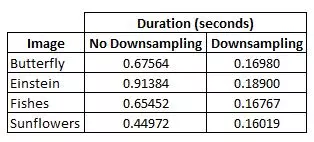
On average, the down sampling method took 26% of the time of the no downsampling method. This performance bonus will only increase as the size of the image and filter increase. This is a very efficient implementation.
Other minor notes include the use of an odd kernel size in order to avoid shifting artifacts and bi-cubic interpolation to keep spatial resolution up at the cost of a little bit of time performance.
function [ scaleSpace ] = generateScaleSpace( img_GrayScale, numScales, sigma, scaleMultiplier, bShouldDownsample )
%GENERATESCALESPACE Summary of this function goes here
%   Detailed explanation goes here

    [h,w] = size(img_GrayScale);
    scaleSpace = zeros(h, w, numScales); % structure to hold the scale space

    %Applying the kernel filter is all about relative size (between the
    %kernel and the image). Conceptually we want to increase the kernel
    %size and reapply it to the image to generate the different scales.
    %But it is relatively inefficient to repeatedly filter the image with
    %a kernel of increasing size. Instead of increasing the kernel size by
    %a factor of k, simply downsample the image by a factor 1/k and apply
    %the same kernel. Of course after applying the kernel, the result the
    %result has to be upsampled.

    if bShouldDownsample
        % Process will be... don't change filter size, but downsize the image
        %by 1/k, filter with same kernel, and then rescale/upsize back

        %-------- Generate just 1 normalized filter (min size 1x1)-------------
        %(borrowed mostly from "http://slazebni.cs.illinois.edu/spring16/harris.m")
        kernelSize = max(1,fix(6*sigma)+1);  %+1 to guarantee odd filter size
        % Create a Laplacian of Gaussian kernel ('log')
        LoGKernel = fspecial( 'log', kernelSize, sigma );
        % Nomrmalize the kernel
        LoGKernel = sigma.^2 * LoGKernel;

        reUpscaledImg = zeros(h,w);
        downsizedImg = img_GrayScale;


        for i = 1:numScales
            % Downsize the image by 1/k... use bicubic instead of bilinear to
            % keep spatial resolution. Here k is the scaleMultiplicationConstant
            if i==1
                downsizedImg = img_GrayScale;
            else
                downsizedImg = imresize(img_GrayScale, 1/(scaleMultiplier^(i-1)), 'bicubic');
            end
            % Filter the image to generate a response to the laplacian of
            % gaussian
            filteredImage = imfilter(downsizedImg, LoGKernel,'same', 'replicate');
            %Save square of Laplacian response for current level of scale space
            filteredImage = filteredImage .^ 2;

            % Upscale the filter response
            reUpscaledImg = imresize(filteredImage, [h,w], 'bicubic');
            % Store it at the appropriate level in the scale space
            scaleSpace(:,:,i) = reUpscaledImg;
        end
    else
        %increase the kernel size and reapply it to the image
        %to generate the different scales.
        for i = 1:numScales
            %--Calculate a new sigma, and regenerate the kernel for each scale
            scaledSigma = sigma * scaleMultiplier^(i-1);
            kernelSize = max(1,fix(6*scaledSigma)+1);  %+1 to guarantee odd filter size
            % Create a Laplacian of Gaussian kernel ('log')
            LoGKernel = fspecial( 'log', kernelSize, scaledSigma );
            % Nomrmalize the kernel
            LoGKernel = scaledSigma.^2 * LoGKernel;

            % Filter the image to generate a response to the laplacian of
            % gaussian
            filteredImage = imfilter(img_GrayScale, LoGKernel,'same', 'replicate');
            % Save square of Laplacian response for current level of scale space
            filteredImage = filteredImage .^ 2;

            % Store it at the appropriate level in the scale space
            scaleSpace(:,:,i) = filteredImage;
        end
    end

end
Two Dimensional Non-Maximum Suppression
To perform nonmaximum suppression in scale space, its easiest to first do nonmaximum suppression in each 2D slice separately. The following code performs a 2 dimensional non-maximum suppression. It makes use of the ordfilt2 Matlab function for most of the busy work.
function [ img_2D_NMS ] = nms_2D( img, radius )
% Extract local maxima
%   Detailed explanation goes here
    neighborhoodSize = 2*radius+1; %size of mask
    domain = ones(3,3);

    img_2D_NMS = ordfilt2(img, neighborhoodSize^2, domain);
end
Three Dimensional Non-Maximum Suppression
After each slice has been non-max suppressed, a 3D non-max suppression can be performed in the entire scale space. This is best done by comparing a neighborhood of slices (in this case 3) and keeping only the local max between neighboring slices. In this way there can still be multiple local maxima at a given pixel location if they are separated by at least 1 scale. This would manifest as nested circles in the final output markers.
function [ scaleSpace_3D_NMS ] = nms_3D( scaleSpace_2D_NMS, originalScaleSpace, numScales )
%NMS_3D Summary of this function goes here
%   Detailed explanation goes here\

[h,w] = size(scaleSpace_2D_NMS(:,:,1));
maxVals_InNeighboringScaleSpace = scaleSpace_2D_NMS;
for i = 1:numScales
    if i == 1
        lowerScale = i;
        upperScale = i+1;
    elseif i < numScales
        lowerScale = i-1;
        upperScale = i+1;
    else
        lowerScale = i-1;
        upperScale = i;
    end
    %each row and column holds the maximum value at that row and col from
    %the neighboring scale space...
    %ie: the maximum of the value at pix x,y in the scale space above,
    %current and below... so neighboring scales will end up with the same
    %values at many row and col positions... this is an intermediate calc
    maxVals_InNeighboringScaleSpace(:,:,i) = max(maxVals_InNeighboringScaleSpace(:,:,lowerScale:upperScale),[],3);
end

%mark every location where the max value is the actualy value from that
%scale with a 1, and a 0 otherwise. (Binary flag)
originalValMarkers = maxVals_InNeighboringScaleSpace == originalScaleSpace;
%only keep the max vals that were actually from those locations
scaleSpace_3D_NMS = maxVals_InNeighboringScaleSpace .* originalValMarkers;

end
Retrieving Positions and Characteristic Scales of Blobs
Here the marker positions and radii are determined so that they may be overlaid on top of the original image. The ‘find’ function is used to extract final nozero values (corresponding to detected regions).
function [ radiiByScale ] = calcRadiiByScale( numScales, scaleMultiplier, sigma )
%CALCRADIIBYSCALE Summary of this function goes here
%   Detailed explanation goes here

    radiiByScale = zeros(1,numScales);
    for i = 1:numScales
        radiiByScale(i) =  sqrt(2) * sigma * scaleMultiplier^(i-1);
    end
end
function [ blobMarkers ] = retrieveBlobMarkers( scaleSpace, radiiByScale  )
%RETRIEVEBLOBMARKERS Summary of this function goes here
%   Detailed explanation goes here

    [h,w,numScales] = size(scaleSpace);
    blobMarkers = [];
    for i = 1:numScales
        %find indices in the scale slice where the pixel value != 0
        %(assumes prior thresholding)
        [newMarkerRows, newMarkerCols] = find(scaleSpace(:,:,i));

        %create a 3xNumMarkers matrix where row 1 = x pos, row 2 = y pos,
        %row 3 = radius
        newMarkers = [newMarkerCols'; newMarkerRows'];
        newMarkers(3,:) = radiiByScale(i);

        %append the calculated positions/radius for this slice to the
        %entire collection (transpose of course)
        blobMarkers = [blobMarkers; newMarkers'];
    end

end
More Results
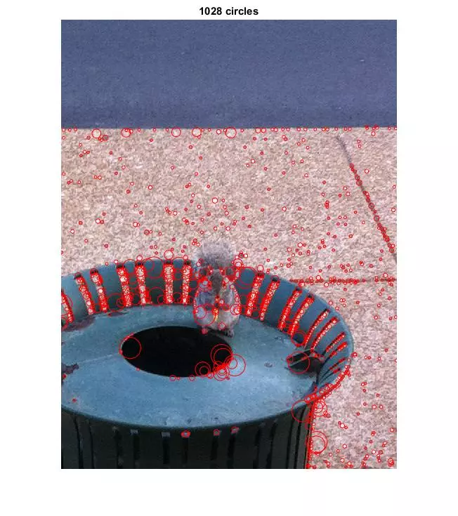
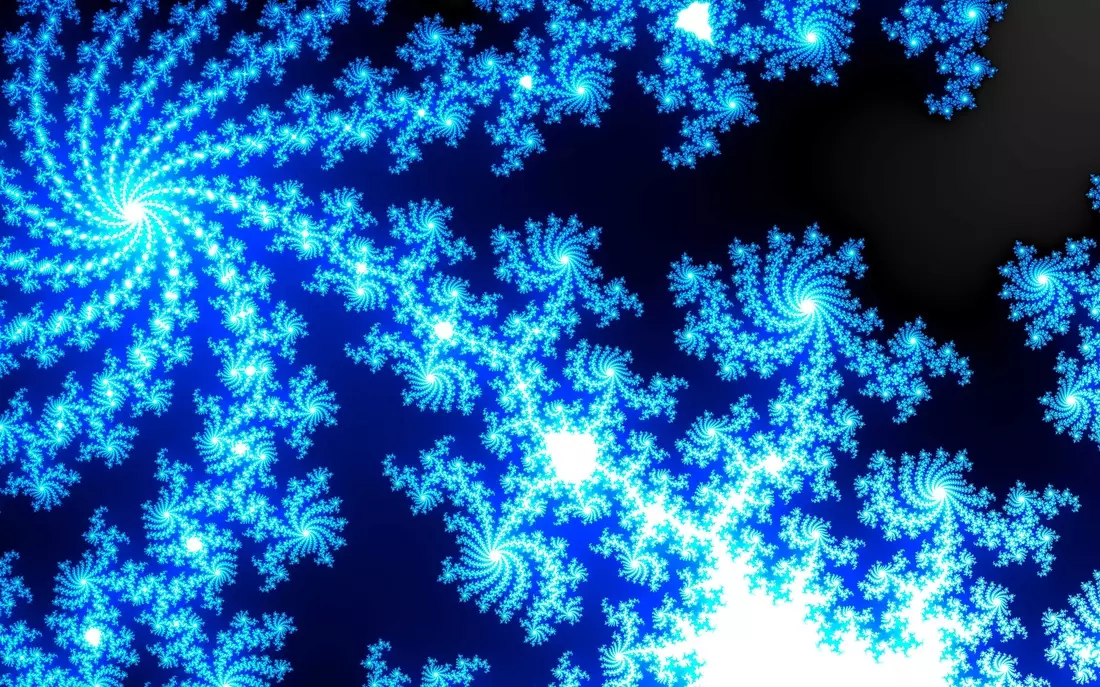
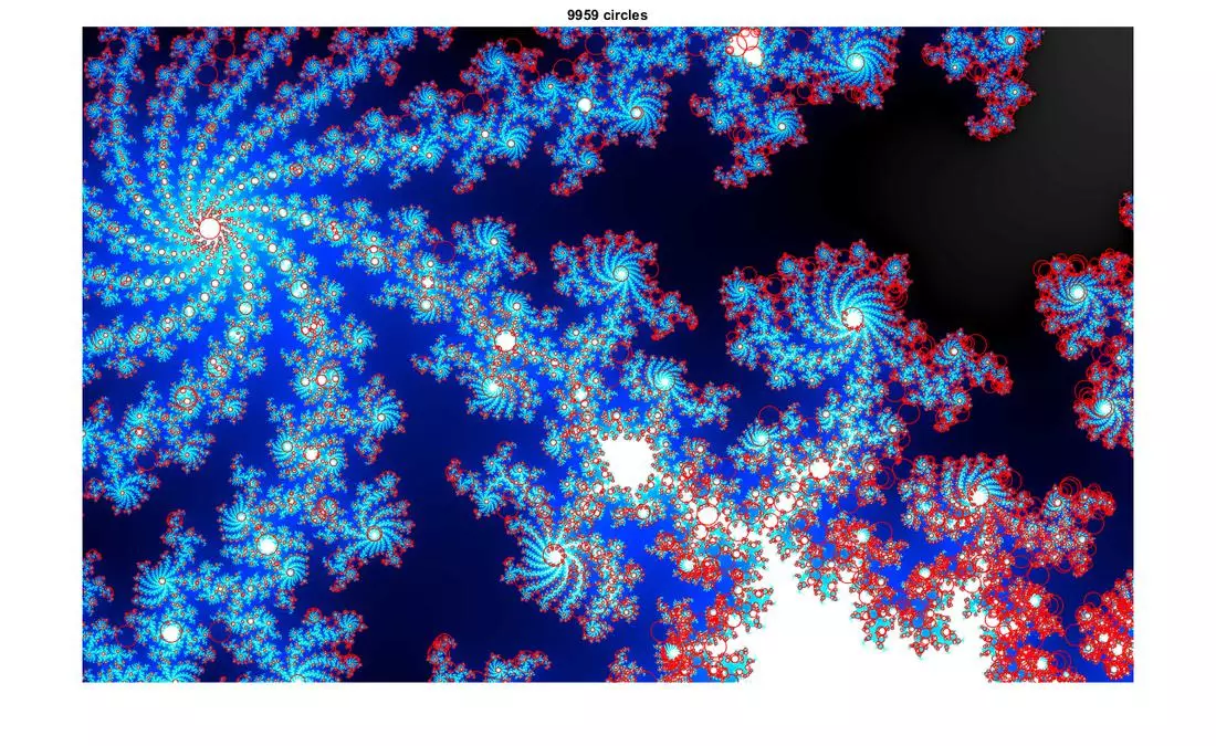
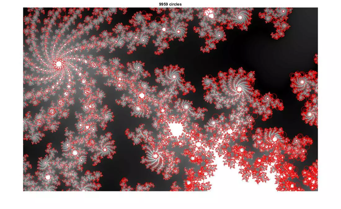


Comments