Estimating Homography w/ RANSAC
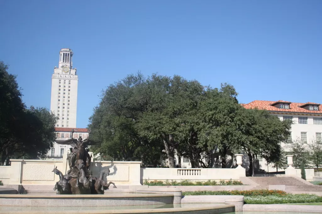
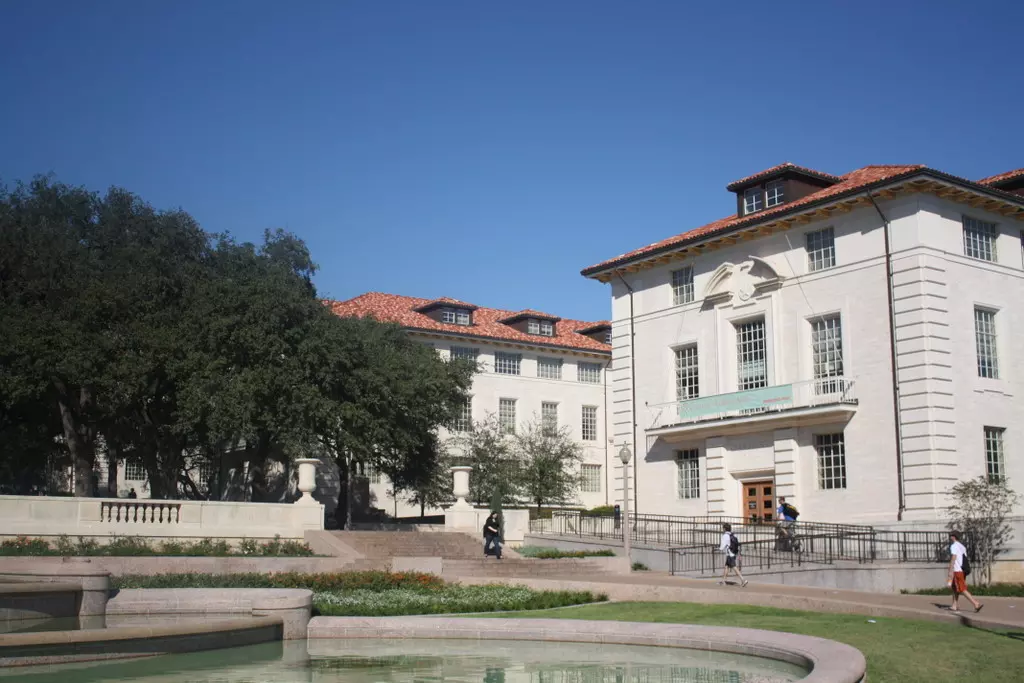
The main goal is to implement robust homography and fundamental matrix estimation to register pairs of images separated either by a 2D or 3D projective transformation. This page details the estimation of homography. Another page coming soon will detail the estimation of the fundamental matrix.
The source code can be obtained here: github.com/dcyoung/ImageAlign
Fitting a Homography (Provided Known Matches)
To be brief, the homography matrix is the transformation between two views of a planar surface OR between two images from cameras that share the same center. If parallel lines were somehow preserved, one could estimate this with 3 points… as 3 points are all that is needed to describe a parallelogram. However, homography describes a transform of a quadrilateral into any other quadrilateral. With an unrestricted quadrilateral, 4 points (4 matches for a total of 8 points to be more specific) are required for estimation. There are 2 linearly independent equations per match. All the equations are stacked into the 8x9 matrix “A” such that Ah=0, where h is a column vector of 9 values that make up the 3x3 H matrix. H has 9 parameters, but only 8 D.O.F. because the scale is arbitrary. Each match yields 2 linearly independent equations, so only 4 matches are required to estimate H. Finding the H matrix from Ah = 0 calls for homogenous least squares, ie: finding the h which minimizes ||A*h||^2. This can be accomplished by setting h to the eigenvector of A’A corresponding to the smallest eigenvalue. In Matlab the solution can be obtained from the SVD of A by the singular vector corresponding to the smallest singular value.
function H = fit_homography(pts1_homogenous, pts2_homogenous)
%FIT_HOMOGRAPHY Summary of this function goes here

    if size(pts1_homogenous) ~= size(pts2_homogenous)
        error('Number of matched features in the subset supplied to fit_homography does not match for both images')
    end

    [numMatches, ~] = size(pts1_homogenous);

    %create the A matrix
    A = []; % will be 2*numMatches x 9
    for i = 1:numMatches
        %assume homogenous versions of all the feature points
        p1 = pts1_homogenous(i,:);
        p2 = pts2_homogenous(i,:);

        % 2x9 matrix to append onto A.
        A_i = [ zeros(1,3)  ,   -p1     ,   p2(2)*p1;
                    p1      , zeros(1,3),   -p2(1)*p1];
        A = [A; A_i];
    end

    %solve for A*h = 0
    [~,~,eigenVecs] = svd(A); % Eigenvectors of transpose(A)*A
    h = eigenVecs(:,9);     % Vector corresponding to smallest eigenvalue
    H = reshape(h, 3, 3);   % Reshape into 3x3 matrix
    H = H ./ H(3,3);        % Divide through by H(3,3)

end
Generalized RANSAC
I wrote a function to perform RANSAC but left it slightly general, as I intend to use it in a different project later for estimating the fundamental matrix.
function [ bestFitModel, inlierIndices ] = ransac_H( parameters, x, y, fitModelFxn, errorFxn )
%RANSAC_H Summary of this function goes here
%   Detailed explanation goes here

    [numMatches, ~] = size(x);
    numInliersEachIteration = zeros(parameters.numIterations,1);
    storedModels = {};%zeros(parameters.numIterations,3,3);

    for i = 1 : parameters.numIterations;
        %display(['Running ransac Iteration: ', num2str(i)]);

        %select a random subset of points
        subsetIndices = randsample(numMatches, parameters.subsetSize);
        x_subset = x(subsetIndices, :);
        y_subset = y(subsetIndices, :);

        %fit a model to that subset
        model = fitModelFxn(x_subset, y_subset);

        %compute inliers, ie: find all remaining points that are
        %"close" to the model and reject the rest as outliers
        residualErrors = errorFxn(model, x, y);

        inlierIndices = find(residualErrors < parameters.inlierDistThreshold);

        %record the number of inliers
        numInliersEachIteration(i) = length(inlierIndices);

        %keep track of any models that generated an acceptable numbers of
        %inliers. This collection can be parsed later to find the best fit
        currentInlierRatio = numInliersEachIteration(i)/numMatches;
        if currentInlierRatio >=  parameters.minInlierRatio
            %re-fit the model using all of the inliers and store it
            x_inliers = x(inlierIndices, :);
            y_inliers = y(inlierIndices, :);
            storedModels{i} = fitModelFxn(x_inliers, y_inliers);
        end
    end

    %retrieve the model with the best fit (highest number of inliers)
    bestIteration = find(numInliersEachIteration == max(numInliersEachIteration));
    bestIteration = bestIteration(1); %incase there was more than 1 with same value
    bestFitModel = storedModels{bestIteration};

    %recalculate the inlier indices for all points, this was done once before
    %when calculting this model, but it wasn't stored for space reasons.
    %Recalculate it now so that it can be returned to the caller
    residualErrors = errorFxn(bestFitModel, x, y);
    inlierIndices = find(residualErrors < parameters.inlierDistThreshold);
end
Estimating Homography using RANSAC
Calling the RANSAC for homography (parameters)
If we somehow had ground truth matches, the homography matrix H could be fit directly without any need for RANSAC. This was covered above. Unfortunately, more often than not, we don’t know the ground truth matches. If not all the matches are guaranteed to be true, the homography can be estimated using a subset of the top (least distance) putative matches. RANSAC is used for this estimation and it works like this:
- Pick 4 matches at random
- Estimate homography from the 4 matches
- Look for additional inliers. That is, apply the estimated homogrpahy transform to points from 1 image and compare with points in other image to see if the distance is below some threshold. If so, its an inlier. If not, its an outlier.
- Repeat multiple times
- Return the homography estimate that yielded the most inliers.
The following function uses the generalized RANSAC (written above) and the homography fitting function (also written above) to estimate the homography matrix. The necessary 4 matches are defined by “parameters.subsetSize” indicating that RANSAC should use 4 matches to estimate the homography. The two function handles passed to the RANSAC are the custom functions written to fit and error test a homography model using 4 pairs of matching data points.
function [ H, inlierIndices ] = estimate_homography( img1Feat, img2Feat )
%ESTIMATE_HOMOGRAPHY Summary of this function goes here
%   Detailed explanation goes here

    parameters.numIterations = 150;      %the number of iterations to run
    parameters.subsetSize = 4;          %number of matches to use each iteration
    parameters.inlierDistThreshold = 10;   %the minimum distance for an inlier
    parameters.minInlierRatio = .3;     %minimum inlier ratio required to store a fitted model

    [H, inlierIndices] = ransac_H(parameters, img1Feat, img2Feat, @fit_homography, @calc_residuals);

    display('Number of inliers:');
    display(length(inlierIndices));
    display('Average residual for the inliers:')
    display(mean(calc_residuals(H, img1Feat(inlierIndices,:), img2Feat(inlierIndices,:))));
end
Calculating Residual Errors
The residual error is calculated here, and is used to error test a fit homography model. This will help RANSAC determine which matches are inliers or outliers given a homography estimate.
function residuals = calc_residuals(H, homoCoord1, homoCoord2)
%CALC_RESIDUALS Summary of this function goes here
%   Detailed explanation goes here

    %transform the points from img 1 by multiplying the homo coord by H
    transformedPoints = homoCoord1 * H;

    %divide each pt by 3rd coord (scale factor lambda) to yield [x;y;1]
    %before taking difference
    lambda_t =  transformedPoints(:,3); %scale factor
    lambda_2 = homoCoord2(:,3);    %scale factor
    cartDistX = transformedPoints(:,1) ./ lambda_t - homoCoord2(:,1) ./ lambda_2;
    cartDistY = transformedPoints(:,2) ./ lambda_t - homoCoord2(:,2) ./ lambda_2;
    residuals = cartDistX .* cartDistX + cartDistY .* cartDistY;
end
Applied Example (stitching images)
Here, 2 images that share the same camera center are supplied to a script which does the following:
- finds features
- describes features
- identifies matches
- estimates homogrpahy using ransac
- warps one image using the estimated homography
- stitches the images together


Main Script
The following script provides an example of how to use all the written functions to estimate a homography matrix.
%Clean up the console and workspace
clear all; clc;

%%%%%%%%%%%%%%%%%%
% Load both images
%%%%%%%%%%%%%%%%%%
img1Filename = 'uttower_left.JPG';
img2Filename = 'uttower_right.JPG';
colorImg1 = imread(img1Filename);
colorImg2 = imread(img2Filename);

%%%%%%%%%%%%%%%%%%%%%%%%%%%%%%%%%%%%
% Convert to double and to grayscale
%%%%%%%%%%%%%%%%%%%%%%%%%%%%%%%%%%%%
colorImg1 = im2double(colorImg1);
colorImg2 = im2double(colorImg2);
[heightImg1, widthImg1, ~] = size(colorImg1);
[heightImg2, widthImg2, ~] = size(colorImg2);

grayImg1 = rgb2gray(colorImg1);
grayImg2 = rgb2gray(colorImg2);

%%%%%%%%%%%%%%%%%%%%%%%%%%%%%%%%%%%%%%
% Detect feature points in both images
%%%%%%%%%%%%%%%%%%%%%%%%%%%%%%%%%%%%%%
[r1, c1, r2, c2] = detect_features(grayImg1, grayImg2);

%display an overlay of the features ontop of the image
figure; imshow([colorImg1 colorImg2]); hold on; title('Overlay detected features (corners)');
hold on; plot(c1,r1,'ys'); plot(c2 + widthImg1, r2, 'ys');

%%%%%%%%%%%%%%%%%%%%%%%%%%%%%%%%%%%%%%%%%%%%%%%%%%%%%%%%%%%%%%%%%%
% Extract local neighborhoods around every keypoint in both images
%%%%%%%%%%%%%%%%%%%%%%%%%%%%%%%%%%%%%%%%%%%%%%%%%%%%%%%%%%%%%%%%%%
%Specify the size of the neighboring region to be described
neighborhoodRadius = 20;

% Form descriptors simply by "flattening" the pixel values in each
% neighborhood to one-dimensional vectors
featDescriptions_1 = describe_features(grayImg1, neighborhoodRadius, r1, c1);
featDescriptions_2 = describe_features(grayImg2, neighborhoodRadius, r2, c2);

%%%%%%%%%%%%%%%%
% Match Features
%%%%%%%%%%%%%%%%
numMatches = 200;
[img1_matchedFeature_idx, img2_matchedFeature_idx] = match_features(numMatches, featDescriptions_1, featDescriptions_2);

match_r1 = r1(img1_matchedFeature_idx);
match_c1 = c1(img1_matchedFeature_idx);
match_r2 = r2(img2_matchedFeature_idx);
match_c2 = c2(img2_matchedFeature_idx);

% Display an overlay of these best matched features on top of the images
figure; imshow([colorImg1 colorImg2]); hold on; title('Overlay top matched features');
hold on; plot(match_c1, match_r1,'ys'); plot(match_c2 + widthImg1, match_r2, 'ys');

% Display lines connecting the matched features
plot_r = [match_r1, match_r2];
plot_c = [match_c1, match_c2 + widthImg1];
figure; imshow([colorImg1 colorImg2]); hold on; title('Mapping of top matched features');
hold on;
plot(match_c1, match_r1,'ys');           %mark features from the 1st img
plot(match_c2 + widthImg1, match_r2, 'ys'); %mark features from the 2nd img
for i = 1:numMatches             %draw lines connecting matched features
    plot(plot_c(i,:), plot_r(i,:));
end

%%%%%%%%%%%%%%%%%%%%%
% Estimate Homography
%%%%%%%%%%%%%%%%%%%%%
%create homogenous versions of the the matched feature points for each img
img1MatchFeatPts = [match_c1, match_r1, ones(numMatches,1)];
img2MatchFeatPts = [match_c2, match_r2, ones(numMatches,1)];
[H, inlierIndices] = estimate_homography(img1MatchFeatPts,img2MatchFeatPts);
%display(H);
Detecting Feature
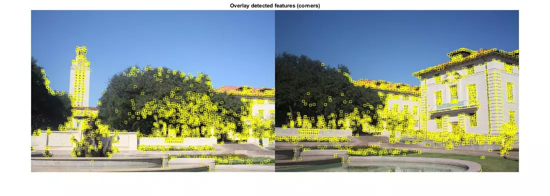
A harris corner detector was used to detect features.
function [ r1, c1, r2, c2 ] = detect_features( grayImg1, grayImg2 )
%DETECT_FEATURES Summary of this function goes here
%   Detailed explanation goes here

    %use harris corner detector
    points1 = detectHarrisFeatures(grayImg1);
    points2 = detectHarrisFeatures(grayImg2);

    %extract the pixel locations from the features
    [r1, c1] = deal( zeros(length(points1),1) );
    [r2, c2] = deal( zeros(length(points2),1) );
    for i = 1: length(points1)
        cornerLoc = points1(i).Location;
        r1(i) = round(cornerLoc(2));
        c1(i) = round(cornerLoc(1));
    end
    for i = 1: length(points2)
        cornerLoc = points2(i).Location;
        r2(i) = round(cornerLoc(2));
        c2(i) = round(cornerLoc(1));
    end
end
Describing Features
The following code extracts local neighborhoods around every keypoint in an image, and forms descriptors simply by “flattening” the pixel values in each neighborhood to a one-dimensional vector. The descriptors are normalized to have zero mean an unit standard deviation.
function [ featDescriptions ] = describe_features( img, radius, r, c )
%DESCRIBE_FEATURES Summary of this function goes here
%   Detailed explanation goes here

    numFeat = length(r); %number of features
    featDescriptions = zeros(numFeat, (2 * radius + 1)^2);

    % matrix with a single 1 in the center and zeros all around it
    padHelper = zeros(2 * radius + 1);
    padHelper(radius + 1, radius + 1) = 1;

    % use the pad Helper matrix to pad the img such that the border values
    % extend out by the radius
    paddedImg = imfilter(img, padHelper, 'replicate', 'full');

    %Extract the neighborhoods around the found features
    for i = 1 : numFeat
        %Determine the rows and cols that will make up the neighorhood around
        %the feature. Recall that the padding has offset the indices of the
        %features in the img.. so now, the indices held in r,c can be used as
        %the top left corner of the neighborhood rather than its center
        rowRange = r(i) : r(i) + 2 * radius;
        colRange = c(i) : c(i) + 2 * radius;
        neighborhood = paddedImg(rowRange, colRange);
        flattenedFeatureVec = neighborhood(:);
        featDescriptions(i,:) = flattenedFeatureVec;
    end

    %Normalize all descriptors to have zero mean and unit standard deviation
    featDescriptions = zscore(featDescriptions')';
end
Matching Features
Putative matches are selected based on the matrix of pairwise descriptor distances returned by a borrowed function “dist2” also shown below.

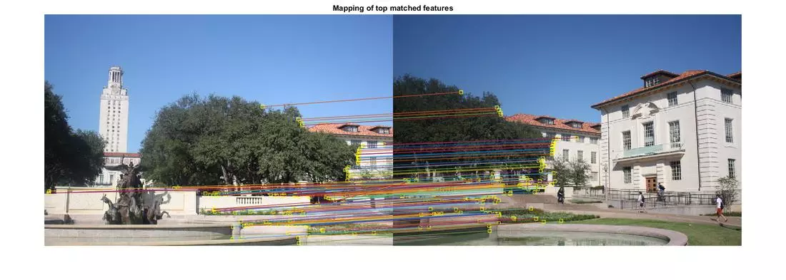
function [ img1Feature_idx, img2Feature_idx ] = match_features( numMatches, featDescriptions_1, featDescriptions_2)
%MATCH_FEATURES Summary of this function goes here
%   Detailed explanation goes here

    %determine the dist between every pair of features between images
    %(ie: every combination of 1 feature from img1 and 1 feature from img2)
    distances = dist2(featDescriptions_1, featDescriptions_2);
    %sort these distances
    [~,distance_idx] = sort(distances(:), 'ascend');
    %select the smallest distances as the best matches
    bestMatches = distance_idx(1:numMatches);
    % Determine the row,col indices in the distances matrix containing the best
    % matches, as they'll be used to determine which feature pair produced that
    % distance. The distances matrix is m x n where m = numFeaturesImg1 and
    % n = numFeaturesImg2... so we access img1 feature as the row and img2
    % feature as the col
    [rowIdx_inDistMatrix, colIdx_inDistMatrix] = ind2sub(size(distances), bestMatches);
    img1Feature_idx = rowIdx_inDistMatrix;
    img2Feature_idx = colIdx_inDistMatrix;
end
The borrowed function for squared distance.
function n2 = dist2(x, c)
% DIST2	Calculates squared distance between two sets of points.
% Adapted from Netlab neural network software:
% http://www.ncrg.aston.ac.uk/netlab/index.php
%
%	Description
%	D = DIST2(X, C) takes two matrices of vectors and calculates the
%	squared Euclidean distance between them.  Both matrices must be of
%	the same column dimension.  If X has M rows and N columns, and C has
%	L rows and N columns, then the result has M rows and L columns.  The
%	I, Jth entry is the  squared distance from the Ith row of X to the
%	Jth row of C.
%	Copyright (c) Ian T Nabney (1996-2001)

    [ndata, dimx] = size(x);
    [ncentres, dimc] = size(c);
    if dimx ~= dimc
        error('Data dimension does not match dimension of centres')
    end

    n2 = (ones(ncentres, 1) * sum((x.^2)', 1))' + ...
      ones(ndata, 1) * sum((c.^2)',1) - ...
      2.*(x*(c'));

    % Rounding errors occasionally cause negative entries in n2
    if any(any(n2<0))
      n2(n2<0) = 0;
end
Estimated Homography Results
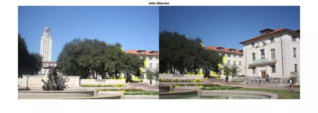
Out of the 200 generated putative matches, 117 inliers were found using the estimate_homography function. The average residual provided the final estimated homography matrix was 1.1855. The image below shows just the inlier matches overlaid on both images.
Warping Image
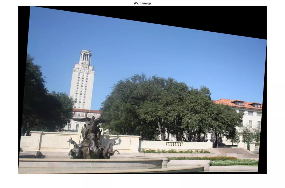
Transforming the first image by applying the estimated homography yields the following transformed image.
% Warp image
homographyTransform = maketform('projective', H);
img1Transformed = imtransform(colorImg1, homographyTransform);
figure, imshow(img1Transformed);title('Warped image');
Stitching Image
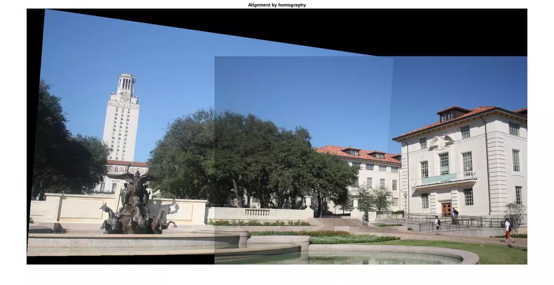
The final stiched composite:

A stitched composite image is generated using the transformed image and the original second image as inputs.
% Stitch the images together with the correct overlap
stitchedCompositeImg = stitch(colorImg1, colorImg2, H);
figure, imshow(stitchedCompositeImg);
title('Alignment by homography');
function [composite] = stitch(im1, im2, H)

    [h1, w1, numChannels1] = size(im1);
    [h2, w2, numChannels2] = size(im2);
    %create a matrix of corner points for the first image
    corners = [ 1 1 1;
                w1 1 1;
                w1 h1 1;
                1 h1 1];
    %warp the corner points using the homography matrix
    warpCorners = homo_2_cart( corners * H );

    %determine the minimum and maximum bounds for the composite image based off
    %the warped corners
    minX = min( min(warpCorners(:,1)), 1);
    maxX = max( max(warpCorners(:,1)), w2);
    minY = min( min(warpCorners(:,2)), 1);
    maxY = max( max(warpCorners(:,2)), h2);

    %use those min and max bounds to define the resolution of the composite image
    xResRange = minX : maxX; %the range for x pixels
    yResRange = minY : maxY; %the range for y pixels

    [x,y] = meshgrid(xResRange,yResRange) ;
    Hinv = inv(H);

    warpedHomoScaleFactor = Hinv(1,3) * x + Hinv(2,3) * y + Hinv(3,3);
    warpX = (Hinv(1,1) * x + Hinv(2,1) * y + Hinv(3,1)) ./ warpedHomoScaleFactor ;
    warpY = (Hinv(1,2) * x + Hinv(2,2) * y + Hinv(3,2)) ./ warpedHomoScaleFactor ;


    if numChannels1 == 1
        %images are black and white... so simple interpolation
        blendedLeftHalf = interp2( im2double(im1), warpX, warpY, 'cubic') ;
        blendedRightHalf = interp2( im2double(im2), x, y, 'cubic') ;
    else
        %images are RGB, so interpolate each channel individually
        blendedLeftHalf = zeros(length(yResRange), length(xResRange), 3);
        blendedRightHalf = zeros(length(yResRange), length(xResRange), 3);
        for i = 1:3
            blendedLeftHalf(:,:,i) = interp2( im2double( im1(:,:,i)), warpX, warpY, 'cubic');
            blendedRightHalf(:,:,i) = interp2( im2double( im2(:,:,i)), x, y, 'cubic');
        end
    end
    %create a blend weight matrix based off the presence of a pixel value from
    %either image in the composite... ie: overlapping region has blendweight of
    %2, a non overlapping region of 1 img has a blendweight of 1, and a region
    %with no img (blank space) has a blendweight of 0.
    blendWeight = ~isnan(blendedLeftHalf) + ~isnan(blendedRightHalf) ;
    %replace all NaN with 0, so they can be blended properly even if there is
    %no pixel value there
    blendedLeftHalf(isnan(blendedLeftHalf)) = 0 ;
    blendedRightHalf(isnan(blendedRightHalf)) = 0 ;
    %add the blendedLeft and Right halves together while dividing by the
    %blendWeight for that pixel.
    composite = (blendedLeftHalf + blendedRightHalf) ./ blendWeight ;

end
Reference Implementation
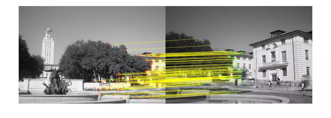
The following is a short script to perform the same operations using commands built into MATLAB’s image processing toolbox. The code written above was an exercise in implementing the algorithms from scratch and not necessarily the most optimized implementations. If you’re looking for good results without worrying about the details, then this simple script will do the same thing.
%%%%%%%%%%%%%%%%%%%%%%%%%%%%%%%%%%%
% Matlab Equivalent (GOLD STANDARD)
%%%%%%%%%%%%%%%%%%%%%%%%%%%%%%%%%%%

%Clean up the console and workspace
clear all;
clc;

% Load both images
img1Filename = 'uttower_left.JPG';
img2Filename = 'uttower_right.JPG';
colorImg1 = imread(img1Filename);
colorImg2 = imread(img2Filename);
% Convert to double and to grayscale
colorImg1 = im2double(colorImg1);
colorImg2 = im2double(colorImg2);
I1 = rgb2gray(colorImg1);
I2 = rgb2gray(colorImg2);

%detect features
points1 = detectHarrisFeatures(I1);
points2 = detectHarrisFeatures(I2);
%describe features
[features1,valid_points1] = extractFeatures(I1,points1);
[features2,valid_points2] = extractFeatures(I2,points2);
%match features
indexPairs = matchFeatures(features1,features2);

matchedPoints1 = valid_points1(indexPairs(:,1),:);
matchedPoints2 = valid_points2(indexPairs(:,2),:);
%display matches
figure; showMatchedFeatures(I1,I2,matchedPoints1,matchedPoints2, 'montage');


Comments