​Estimating Fundamental Matrix ​& Triangulating 3D Points

There were a few goals here. All goals refer to matching points from two images of the same scene from different camera positions.

• Fit a fundamental matrix to the known matches using both the normalized and unnormalized versions of the 8-point algorithm.
• Estimate the fundamental matrix from putative matches using RANSAC and the normalized 8-point algorithm.
• Find the centers of cameras from known camera matrices.
• Use linear least squares to triangulate the position of each matching pair of points given two cameras. Display these two camera centers and reconstructed points in 3D.

The source code can be obtained here: github.com/dcyoung/FundamentalMatrixEstimation

Fitting a Fundamental Matrix (Provided Known Matches)

The following function was written to to fit a fundamental matrix using either the normalized or un-normalized 8 point algorithm.

function [ F ] = fit_fundamental( matches, bShouldNormalize )
%FIT_FUNDAMENTAL Summary of this function goes here
%Output...
%   F: Fundamental Matrix
%Inputs...
%   matches:
%       This is a N x 4 file where the first two numbers of each row
%       are coordinates of corners in the first image and the last two
%       are coordinates of corresponding corners in the second image: 
%       matches(i,1:2) is a point in the first image
%       matches(i,3:4) is a corresponding point in the second image
%   bShouldNormalize:
%       Whether or not the points should be normalized prior to estimating 
%       the fundamental matrix

    %homogenize the points
    x1 = cart_2_homo( matches(:,1:2) );
    x2 = cart_2_homo( matches(:,3:4) );
    
    if bShouldNormalize
        [transform_1, x1_norm] = normalize_coordinates(x1);
        [transform_2, x2_norm] = normalize_coordinates(x2);
        x1 = x1_norm;
        x2 = x2_norm;
    end
    
    u1 = x1(:,1);
    v1 = x1(:,2);
    u2 = x2(:,1);
    v2 = x2(:,2);
   
    %group at least 8 known matches together in a useful form
    temp = [ u2.*u1, u2.*v1, u2, v2.*u1, v2.*v1, v2, u1, v1, ones(size(matches,1), 1)];
    %Obtain an estimate for F by solving the homogenous linear system using
    %those matches
    %display('Solving homogenous linear system');
    [~,~,V] = svd(temp);
    f_vec = V(:,9);
    
    F = reshape(f_vec, 3,3); %reshape the 9x1 vec into the 3x3 fund matrix
    F = rank_2_constraint(F); %enforce the rank 2 constraint on F
    
    if bShouldNormalize
        %if F was computed from normalized points, transform it back to
        %the original coordinates
        F = transform_2' * F * transform_1;
    end
end

The linear system to be solved will have terms that involve a product between feature coordinates. If the coordinates are large, then F could end up w/ values that are orders of magnitude different from one another. This could yield poor behavior in practice. So it is best to do the following:

• normalize the coordinates
• compute F in the normalized coordinates
• adjust it back to the original coordinates later using the normalization transformations

​The following function handles normalization for the normalized 8 point algorithm. The transform is passed back to the caller so that the F matrix may be transformed after fitting.

function [ transform, normCoord ] = normalize_coordinates( homoCoord )
%NORMALIZE_COORDINATES Summary of this function goes here
%   Detailed explanation goes here

    center = mean(homoCoord(:,1:2)); 
    
    offset = eye(3);
    offset(1,3) = -center(1); %-mu_x
    offset(2,3) = -center(2); %-mu_y

    sX= max(abs(homoCoord(:,1)));
    sY= max(abs(homoCoord(:,2)));
    
    scale = eye(3);
    scale(1,1)=1/sX;
    scale(2,2)=1/sY;          
                
    transform = scale * offset;
    normCoord = (transform * homoCoord')';
end

Also a function was written to enforce the rank2 constraint for the F matrix.

function [ rank2_mat ] = rank_2_constraint( mat )
%RANK_2_CONSTRAINT Enforce a rank 2 constraint on 3x3 input matrix
%   Detailed explanation goes here

    %display('Enforcing Rank 2 Constraint');
    %take the svd of the input matrix
    [U, S, V] = svd(mat);
    %throw out the smallest singular value
    S(end) = 0;
    %recalcualte the matrix to yield the closest rank 2 constraint of the
    %original
    rank2_mat = U*S*V';
end

To gauge the quality of the fit model, the following function was written to calculate the the mean squared distance in pixels between points in both images and the corresponding epipolar lines.

function residuals = calc_residuals(F, matches)
%CALC_RESIDUALS Summary of this function goes here
%   Detailed explanation goes here
   
    numMatches = size(matches,1);
    L = (F * [matches(:,1:2) ones(numMatches,1)]')'; % transform points from 
    % the first image to get epipolar lines in the second image

    % find points on epipolar lines L closest to matches(:,3:4)
    L = L ./ repmat(sqrt(L(:,1).^2 + L(:,2).^2), 1, 3); % rescale the line
    distances = sum(L .* [matches(:,3:4) ones(numMatches,1)],2); %distances from each pt to its line
    
    residuals = abs(distances);
end

Results (Fitting Fundamental)

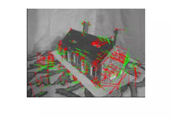
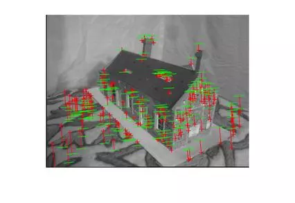
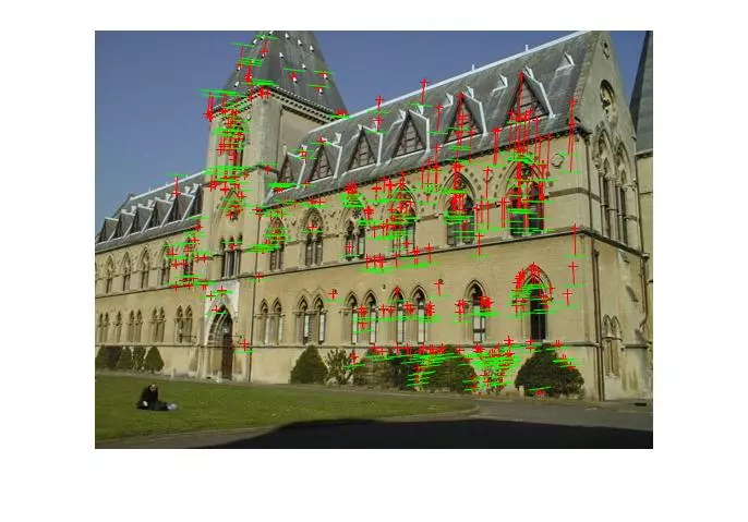
​The following results are for the fitting of a fundamental matrix using known ground truth matches and both the normalized and unnormalized 8 point algorithms. The table shows the mean Residuals for a Fitted F Matrix… ie: the mean squared distance in pixels between points in both images and the corresponding epipolar lines.

Image Set	Normalized	Unnormalized
House	14.5839	26.7532
Library	10.8974	11.8459

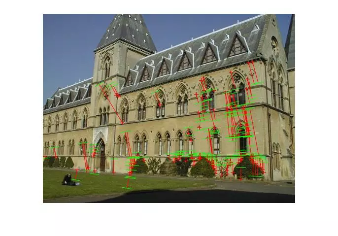
Below, the images show points and segments of corresponding epipolar lines for each image set.

Points and segments of corresponding epipolar lines. Unnormalized (left) and Normalized (right).

Points and segments of corresponding epipolar lines. Unnormalized (left) and Normalized (right).

Generalized RANSAC

I wrote a generalized function to perform RANSAC when I was estimating homography. However some slight tweaks had to be made for estimating the fundamental matrix. The new version is shown below.

function [ bestFitModel, inlierIndices ] = ransac_H( parameters, x, y, fitModelFxn, errorFxn )
%RANSAC_H Summary of this function goes here
%   Detailed explanation goes here

    [numMatches, ~] = size(x);
    numInliersEachIteration = zeros(parameters.numIterations,1);
    storedModels = {};%zeros(parameters.numIterations,3,3);
    
    for i = 1 : parameters.numIterations;
        %display(['Running ransac Iteration: ', num2str(i)]);
        
        %select a random subset of points
        subsetIndices = randsample(numMatches, parameters.subsetSize);
        x_subset = x(subsetIndices, :);
        y_subset = y(subsetIndices, :);
            
        %fit a model to that subset
        model = fitModelFxn(x_subset, y_subset);
        
        %compute inliers, ie: find all remaining points that are 
        %"close" to the model and reject the rest as outliers
        residualErrors = errorFxn(model, x, y);
        
        inlierIndices = find(residualErrors < parameters.inlierDistThreshold);      

        %record the number of inliers
        numInliersEachIteration(i) = length(inlierIndices);
        
        %keep track of any models that generated an acceptable numbers of 
        %inliers. This collection can be parsed later to find the best fit
        currentInlierRatio = numInliersEachIteration(i)/numMatches;
        if currentInlierRatio >=  parameters.minInlierRatio
            %re-fit the model using all of the inliers and store it
            x_inliers = x(inlierIndices, :);
            y_inliers = y(inlierIndices, :);
            storedModels{i} = fitModelFxn(x_inliers, y_inliers);
        end
    end
    
    %retrieve the model with the best fit (highest number of inliers)
    bestIteration = find(numInliersEachIteration == max(numInliersEachIteration));
    bestIteration = bestIteration(1); %incase there was more than 1 with same value
    bestFitModel = storedModels{bestIteration};
    
    %recalculate the inlier indices for all points, this was done once before 
    %when calculting this model, but it wasn't stored for space reasons. 
    %Recalculate it now so that it can be returned to the caller
    residualErrors = errorFxn(bestFitModel, x, y);
    inlierIndices = find(residualErrors < parameters.inlierDistThreshold);
end

Estimating Fundamental Matrix using RANSAC

Calling the RANSAC for fundamental (parameters)

Using an updated version of putative match generation code from before, the fundamental matrix was estimated via RANSAC. A generic implementation of RANSAC was written (above) and was called via the following function, making use of the “fit_fundamental” and “calc_residual” functions already shown. The parameters here just a ballpark. I did not not spend very much time tuning them for performance and there is likely a much better set of general parameters, on top of the need to tune parameters on a case by case basis (for best results).

function [ H, inlierIndices ] = estimate_homography( img1Feat, img2Feat )
%ESTIMATE_HOMOGRAPHY Summary of this function goes here
%   Detailed explanation goes here

    parameters.numIterations = 150;      %the number of iterations to run
    parameters.subsetSize = 4;          %number of matches to use each iteration
    parameters.inlierDistThreshold = 10;   %the minimum distance for an inlier
    parameters.minInlierRatio = .3;     %minimum inlier ratio required to store a fitted model

    [H, inlierIndices] = ransac_H(parameters, img1Feat, img2Feat, @fit_homography, @calc_residuals);
    
    display('Number of inliers:');
    display(length(inlierIndices));
    display('Average residual for the inliers:')
    display(mean(calc_residuals(H, img1Feat(inlierIndices,:), img2Feat(inlierIndices,:))));
end

Results (Estimating Fundamental)

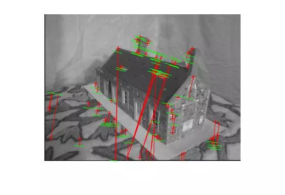
​The following results are for the RANSAC estimation of a fundamental matrix using putative matches and the normalized 8 point algorithm.

Image Set	# of Inliers	# of Starting Matches	Mean Inlier Residual
House	85	100	8.3322
Library	174	200	12.8642

Points and segments of corresponding epipolar lines for the house and library image sets are shown below. The performance has clearly dropped without known matches, but I didn’t spend a lot of time parameter tuning the call to RANSAC and the putative match generation was rather naive.

Triangulation

Calculating Triangulated Points and their Projections

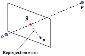
The following snippet calculates the triangulated points and the projected triangulated points onto both images planes. The latter is for the calculation of residuals. What this means is you take the triangulated 3D point (P) and project it onto the image plane of each camera again, using the camera matrix. This reprojection yields new points (p_hat) near the original ones (p). Then, the euclidean distance between the original and reprojected point is calculated in both image planes.

...

%homogenize the coordinates
x1 = cart_2_homo(matches(:,1:2));
x2 = cart_2_homo(matches(:,3:4));
numMatches = size(x1,1);
triangPoints = zeros(numMatches, 3);
projPointsImg1 = zeros(numMatches, 2);
projPointsImg2 = zeros(numMatches, 2);

%calcualte the triangulated points, + their projections onto each img plane
for i = 1:numMatches
    pt1 = x1(i,:);
    pt2 = x2(i,:);
    crossProductMat1 = [  0   -pt1(3)  pt1(2); pt1(3)   0   -pt1(1); -pt1(2)  pt1(1)   0  ];
    crossProductMat2 = [  0   -pt2(3)  pt2(2); pt2(3)   0   -pt2(1); -pt2(2)  pt2(1)   0  ];    
    Eqns = [ crossProductMat1*camMatrix1; crossProductMat2*camMatrix2 ];
    
    [~,~,V] = svd(Eqns);
    triangPointHomo = V(:,end)'; %4 dim (3 dimensions + homo coord)
    %save the triangulated 3d point
    triangPoints(i,:) = homo_2_cart(triangPointHomo);
    
    %project the triangulated point using both camera matrices for later
    %residual calculations
    projPointsImg1(i,:) = homo_2_cart((camMatrix1 * triangPointHomo')');
    projPointsImg2(i,:) = homo_2_cart((camMatrix2 * triangPointHomo')');
    
end

Plotting Triangulation

The following function was written to extract the camera centers from the camera matrices.

function [ cameraCenter ] = get_cam_center( cameraMatrix )
%GET_CAM_CENTER Summary of this function goes here
%   Detailed explanation goes here

    [~, ~, V] = svd(cameraMatrix);
    cameraCenter = V(:,end);
    cameraCenter = homo_2_cart(cameraCenter'); %unhomogenize the point
end

Finally, this function plots the triangulated points and the camera centers in 3d world space.

function [  ] = plot_triangulation( triangPoints, camCenter1, camCenter2 )
%PLOT_TRIANGULATION Summary of this function goes here
%   Detailed explanation goes here

    figure; axis equal;  hold on; 
    plot3(-triangPoints(:,1), triangPoints(:,2), triangPoints(:,3), '.r');
    plot3(-camCenter1(1), camCenter1(2), camCenter1(3),'*g');
    plot3(-camCenter2(1), camCenter2(2), camCenter2(3),'*b');
    grid on; xlabel('x'); ylabel('y'); zlabel('z'); axis equal;
    
end

Results (Triangulation)

The following table shows the residuals between the observed 2D points and the projected 3D points in the two images. See the previous section for a visual representation of what this means.

Image Plane	Mean Dist Between Observed 2D & Projected 3D Point
House Image 1	0.002522
House Image 2	0.15655

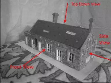
The triangulated points were then plotted in 3 dimensional world space. To make things easier, adopt the following notation for viewing direction. The labeled directions “Front, Side and Top Down” views are shown below.

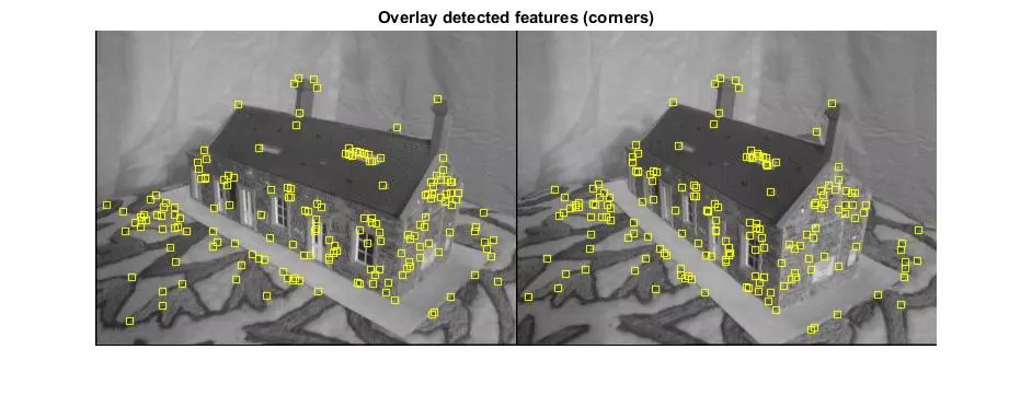
​And make note of the overlaid feature locations.

Now that the reference material is out of the way, here are two slightly different TOP DOWN views of the triangulated points and camera centers from the “house” image set. The triangulated points are shown as red dots. The first camera center is shown as a green star and the second camera center is shown as a blue star.

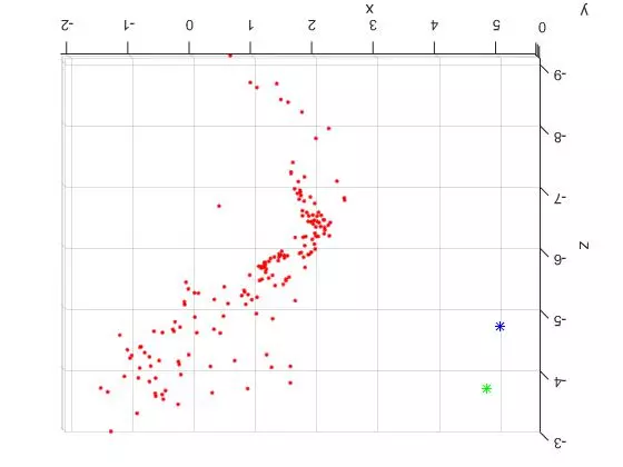
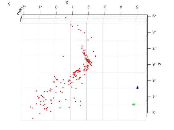
​The large spread out set of points on the lower/left side of the plots are all coplanar features from the tablecloth to the left of the house in the original photos. See the overlaid features images above for reference. Looking at the 3D plots, you can clearly see the corner of the building as the dense “L” shape. And as expected, the position of the second camera center is further to the right (relative to the corner). Because of this, the the blue center can see more of the side view than the green camera center.

Now, here are two additional views of the triangulated points and camera centers from the “house” image set. The “Front Facing” view is shown on the LEFT and the “Side Facing” view is shown on the RIGHT. The plots have been rotated to shown the ground plane of the table as a horizontal line.

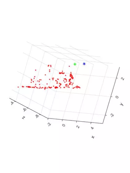
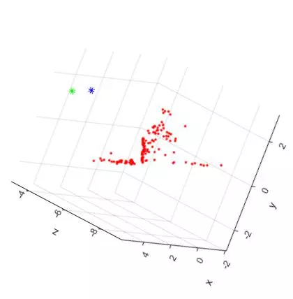
​The additional two views shown the front and side facing views of the house. As expected, the shape of the house can be seen from both angles. Overall, the triangulation and 3D reconstruction of the house image set turned out to be surprisingly accurate.