Comparing Classifiers in R
Dataset
The following writeup compares various classifiers trying to match faces. The training dataset to do with matching faces can be found here: https://courses.engr.illinois.edu/cs498df3/data/pubfig_dev_50000_pairs.txt Each vector consists of a label, followed by measurements of attributes from two faces as produced by some complex vision program. The label indicates if the faces belong to the same class (ie: same person), while the rest of the vector consists of (attribute values for face 1) (attribute values for face 2). The dataset is large (around 100Mb). Various classifiers were trained on this dataset and accuracy was reported on an unknown evaluation set via an online Kaggle competition.
Results
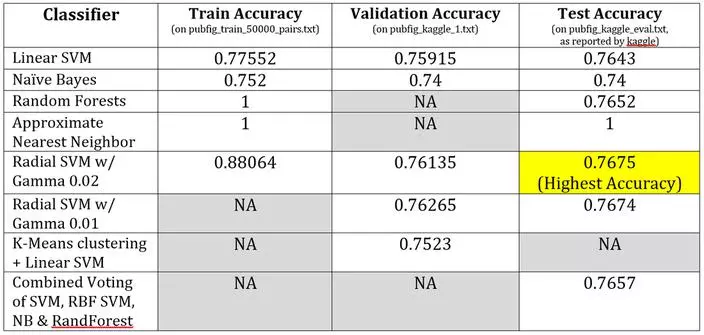
For each of the classifiers below, the training was performed on all data from “pubfig_train_50000pairs.txt”. Where applicable and when time permitted, parameter tuning was performed using the “pubfig_kaggle#.txt” files. The classification accuracy of the trained classifier is shown for the same training data, one example of the validation data, and the test/evaluation data. For the test accuracy, the value was reported by Kaggle as we do not have access to the ground-truth labels.

Implementation
Basic Setup
#------------------------------------- SETUP WORK --------------------------------------
#clear the workspace and console
rm(list=ls())
cat("\014") #code to send ctrl+L to the console and therefore clear the screen

#install packages as necessary:
#install.packages("RANN");
#install.packages("cluster")
#install.packages("stats")

#import libraries
library(klaR)
library(caret)
library(stringr)
library(randomForest)
library(svmlight)
library(RANN) #for finding approximate nearest neighbor
library(cluster)
library(stats)

#----------------------------------------Setup the workspace--------------------------------
setwd('~/WorkingDirectoryNameGoesHere')
Pre-Process Features
The key to an initial performance jump was the pre-processing of features. Each example was made up of two feature vectors, which were replaced by the difference between the two feature vectors (i.e. the scaled Euclidian distance between the two feature vectors in high dimensional space).
###-------------------------------TRAINING DATA---------------------------------------------
#retrieve all the data (each row is 147 items long: 1 label followed by 2x73 feature vectors)
data <- read.table('pubfig_dev_50000_pairs_no_header.txt',sep='\t',header=F);

#grab the labels
labels <- data[,1];
#grab the features (2x 73 features vectors)
features <- matrix(NA,nrow=nrow(data),ncol=(ncol(data)-1)/2);
#features <- data[,-1]; #accuracy: .53

#pre-process the features to yield a single 73 item feature vector that is the scaled euclidian distance between each respective feature
#feature set 1:
features <- scale(abs(as.matrix(data[,2:74]) - as.matrix(data[,75:ncol(data)]))); #accuracy: 0.7684

#feature set 2: feature set 1 + squared values of feature set 1
#features <- scale(abs(as.matrix(data[,2:74]) - as.matrix(data[,75:ncol(data)]))); #accuracy: 0.7684
#features <- cbind(features,features^2);
#sum(features[,74] == features[,1]^2) #checked
Defining Data Partitions
During the initial prototyping of various classifiers, a smaller subset of data was used (~20% -50% of the training dataset). This subset was split into training and testing portions for the various training procedures. Surprisingly, the results from these smaller training sets were better than the final results using the entire training set and the validation sets for testing. For example over 80% accuracy was obtained using an SVM on a smaller training portion split into training and test sets, but 80% accuracy could not be reached with any SVM when training on all the data. This may be due to human bias in selectively reporting our results to ourselves. Prototyping on these smaller sets was necessary however, as re-training a classifier such as the RBF SVM on the entire data set for each of many gamma values would have taken a long time.
###-------------------------------Validation data-------------------------------------------
val_featureData_1 <- read.table('pubfig_kaggle_1.txt', sep='\t', header=F);
val_featureData_2 <- read.table('pubfig_kaggle_2.txt', sep='\t', header=F);
val_featureData_3 <- read.table('pubfig_kaggle_3.txt', sep='\t', header=F);
val_labelsData_1 <- read.table('pubfig_kaggle_1_solution.txt', sep=",", header=F);
val_labelsData_2 <- read.table('pubfig_kaggle_2_solution.txt', sep=",", header=F);
val_labelsData_3 <- read.table('pubfig_kaggle_3_solution.txt', sep=",", header=F);

#grab the labels
val_labels_1 <- val_labelsData_1[,2];
val_labels_2 <- val_labelsData_2[,2];
val_labels_3 <- val_labelsData_3[,2];

val_features_1 <- matrix(NA,nrow=nrow(val_featureData_1),ncol=ncol(val_featureData_1)/2);
val_features_1 <- scale(abs(as.matrix(val_featureData_1[,1:73]) - as.matrix(val_featureData_1[,74:ncol(val_featureData_1)])));

val_features_2 <- matrix(NA,nrow=nrow(val_featureData_2),ncol=ncol(val_featureData_2)/2);
val_features_2 <- scale(abs(as.matrix(val_featureData_2[,1:73]) - as.matrix(val_featureData_2[,74:ncol(val_featureData_2)])));

val_features_3 <- matrix(NA,nrow=nrow(val_featureData_3),ncol=ncol(val_featureData_3)/2);
val_features_3 <- scale(abs(as.matrix(val_featureData_3[,1:73]) - as.matrix(val_featureData_3[,74:ncol(val_featureData_3)])));


###-------------------------------Evaluation/Testing DATA ----------------------------------
eval_featureData <- read.table('pubfig_kaggle_eval.txt', sep='\t', header=F);
eval_features <- matrix(NA,nrow=nrow(eval_featureData),ncol=ncol(eval_featureData)/2);
eval_features <- scale(abs(as.matrix(eval_featureData[,1:73]) - as.matrix(eval_featureData[,74:ncol(eval_featureData)])));


#-------------------------split up the data for testing and training------------------------------

###IF USING THE VALIDATION DATA...
trainingLabels <- labels;
trainingFeatures <- features;
testLabels <- val_labels_1; #val_labels_1; val_labels_2; val_labels_3
testFeatures <- eval_features; #val_features_1; val_features_2; val_features_3;

###IF ONLY USING THE TRAINING DATA... need to split it up into test and train portions
#there is too much data for rapid iteration, use this to scale down how big the initial pool is during prototyping
useDataIndices <- createDataPartition(y=labels, p=.5, list=FALSE);
testDataIndices <- createDataPartition(y=labels[useDataIndices], p=.2, list=FALSE);
trainingLabels <- labels[useDataIndices]; trainingLabels <- trainingLabels[-testDataIndices];
testLabels <- labels[useDataIndices]; testLabels <- testLabels[testDataIndices];
trainingFeatures <- features[useDataIndices,]; trainingFeatures <- trainingFeatures[-testDataIndices,];
testFeatures <- features[useDataIndices,]; testFeatures <- testFeatures[testDataIndices,];
Linear SVM
A linear SVM worked surprisingly well given that the data intuitively seems to extend radially out from an ideal 0 distance. It was not expected that a linear SVM would do so well.
#run an SVM
svm <- svmlight(trainingFeatures,trainingLabels,pathsvm='Path to svm goes here')
predictedLabels<-predict(svm, testFeatures)
foo<-predictedLabels$class #"foo" = class labels (1 or 0) for each item in test set
#get classification accuracy:
accuracy<-sum(foo==testLabels)/(sum(foo==testLabels)+sum(!(foo==testLabels)))
Naive Bayes
The naïve bayes classifier took a long time to train, but performed adequately. It did have the lowest final accuracy.
#run Naive Bayes
model<-train(trainingFeatures, as.factor(trainingLabels), 'nb', trControl=trainControl(method='cv', number=10))
teclasses<-predict(model,newdata=testFeatures)
cm<-confusionMatrix(data=teclasses, testLabels)
accuracy<-cm$overall[1]
Random Forests
The random forest classifier took a long time to train, but performed well. It was nearly as accurate as the SVMs, with a training time somewhere in between the linear SVM and the RBF SVM.
#run Random Forest,
faceforest.allvals <- randomForest(x=trainingFeatures,y=trainingLabels,
                                   xtest=testFeatures,ytest=testLabels);

faceforest.allvals <- randomForest(x=trainingFeatures,y=trainingLabels,
                                   xtest=testFeatures);
predictedLabels <- faceforest.allvals$test$predicted > .5
predictedLabels[predictedLabels] = 1;
predictedLabels[!predictedLabels] = 0;
foo <- predictedLabels;
accuracy<-sum(foo==testLabels)/(sum(foo==testLabels)+sum(!(foo==testLabels)))
Approximate Nearest Neighbors
The classification strategy using nearest neighbors (comparison of labels from the lookup table) was guaranteed to yield 100% accuracy. The question was whether an approximate nearest neighbor package could yield nearly the same performance as a nearest neighbor package. The results would indicate yes. The training accuracy and the testing accuracy were both 100%. This would indicate the correct nearest neighbor was being accurately selected via the approximate algorithm, and significantly faster.
#######################
#Part 2: Approximate Nearest Neighbors
#######################
# -have a reference dictionary of people (names) and many images of that person's face represented as attribute vectors
# -want to determine if two feature vectors represent face images of the same person...
# -will use the reference dictionary as a lookup table, and simply find the nearest neighbor
#   (in this case exact same feature vector) from the dictionary for both of the example's
#   feature vectors. Compare the labels (names) of each found neighbor and see if they're the same name.
# -expect 100% accuracy here with a nearest neighbors classifier, but how close can we get to 100% with an
#   approximate nearest neighbors package? Answer: basically 100%.
# - Purpose: to demonstrate that approximate nearest neighbors can work just about the same as nearest neighbors

#retrieve the reference dictionary of names and associated face images
namedata <- read.table("pubfig_attributes.txt",header=F,sep="\t");
namedata.att <- namedata[,-c(1:2)];

n <- 10000;
face1.nn <- nn2(namedata.att,data[1:n,2:74],k=1);
face2.nn <- nn2(namedata.att,data[1:n,75:ncol(data)],k=1);

predicted <- namedata[face1.nn$nn.idx,1] == namedata[face2.nn$nn.idx,1]; #creates a boolean vector
predicted[predicted] = 1; #turn that boolean vector into 0's and 1's
accuracy = sum(data[1:n,1] == predicted) / length(predicted);
print(accuracy)


#using the evaluation data...

#retrieve the reference dictionary of names and associated face images
namedata <- read.table("pubfig_attributes.txt",header=F,sep="\t");
namedata.att <- namedata[,-c(1:2)];

face1.nn <- nn2(namedata.att, eval_featureData[,1:73], k=1);
face2.nn <- nn2(namedata.att, eval_featureData[,74:ncol(eval_featureData)], k=1);

predicted <- namedata[face1.nn$nn.idx,1] == namedata[face2.nn$nn.idx,1]; #creates a boolean vector
predicted[predicted] = 1; #turn that boolean vector into 0's and 1's

accuracy = sum(data[1:n,1] == predicted) / length(predicted);
Radial basis function SVM
A linear SVM worked surprisingly well given that the data intuitively seems to extend radially out from an ideal 0 distance. It was not expected that a linear SVM would do so well. Instead it was predicted that an SVM using a radial-basis-function (RBF) would perform better, which it did. An RBF SVM is capable of choosing a non-linear decision boundary by mapping to a higher dimension feature space. But, although the RBF SVM yielded the highest accuracy, the performance gain was minimal and at the cost of significantly longer training time. Both versions of the SVM were tried a second time with appended features equal to the square of the pre-processed feature vector. This did not improve performance, and the results were not generated for the entire dataset so they are absent. Most likely these additional features were not as beneficial given the initial pre-processing.
Most likely the RBF SVM worked well because the data was appropriately pre-processed and the RBF SVM somewhat subsumes both the linear and polynomial variants of an SVM classifier. Unfortunately the slightly better performance is not likely worth the much longer training time required by the RBF SVM.
#run a radial basis kernal SVM (in theory, should subsume both linear or polynomial)
svm <- svmlight(trainingFeatures,trainingLabels, svm.options = "-t 2 -g .03", pathsvm='Path to svm goes here')
predictedLabels<-predict(svm, testFeatures)
foo<-predictedLabels$class #"foo" = class labels (1 or 0) for each item in test set
#get classification accuracy:
accuracy<-sum(foo==testLabels)/(sum(foo==testLabels)+sum(!(foo==testLabels)))
Other Variants
Lastly, there was an attempt to implement a classifier defined by a K-Means Clustering with a corresponding SVM for each cluster. But the performance here was right on par with the other SVMs. A voting system didn’t help much, and soft/fuzzy clustering packages did not seem to cooperate for this classifier. Neither approach yielded better performance than the RBF SVM.
#######################
#Other Variant: K Means Clustering + SVMLight
#######################
# Training:
#   -run kmeans clustering on the training data to create k clusters
#   -for each cluster
#     -train a separate svm classifier using the training data in that cluster
#
# Classify a test example:
#   -determine which cluster is closest to the example point
#   -use the svm from that chosen cluster to classify the example point

#accuracy at k = 5, 50% of dataset used, 20% test 80% train was 0.7614


k = 5;  #number of clusters to use... recall that there are only two classes
kmeans.train.output <- kmeans(trainingFeatures,centers=k);

#the trainingLabels are provided as 0 and 1, but the svm wants them to map to -1 and 1... so convert 0's to -1
trainingLabels[trainingLabels==0] = -1;
testLabels[testLabels==0] = -1;

#train an SVM for each cluster
svm_list <- list();
for (i in 1:k){
  svm_list[[i]]<-svmlight(trainingFeatures[kmeans.train.output$cluster==i,], trainingLabels[kmeans.train.output$cluster==i], pathsvm='Path to svm goes here')
}

#select the nearest cluster center for each test example
nearest_cluster_center <- nn2(kmeans.train.output$centers,testFeatures,k=1);


#create a structure to hold the predicted labels of any example near each SVM
predictedLabelsList = vector(mode = "list", length = k);
for(i in 1:k){
  if(sum(nearest_cluster_center$nn.idx==i) > 0){
    predictedLabelsList[[i]] = predict(svm_list[[i]], testFeatures[nearest_cluster_center$nn.idx==i,])
  }
}

#predict the label of the test examples using the svm associated with the nearest cluster to that test example
predictedLabels = rep(NA,nrow(testFeatures));
for(i in 1:k){
  if(sum(nearest_cluster_center$nn.idx==i) > 0 & !is.null(predictedLabelsList[[i]]$class)){
    predictedLabels[nearest_cluster_center$nn.idx==i] = as.numeric(predictedLabelsList[[i]]$class);
  }
}

predictedLabels[predictedLabels==1] = -1;
predictedLabels[predictedLabels==2] = 1;

accuracy = sum(predictedLabels == testLabels)/length(predictedLabels);
print(accuracy)


Comments